Applications et fonctions
Applications et fonctions
Définition d'une application
- Soit et deux ensembles. Une application de dans est la donnée d'une processus de correspondance qui à élément de permet d'associer un élément de . Cet élément est alors noté . L'ensemble est alors appelé ensemble de départ et l'ensemble d'arrivée. Et il est d'usage d'adopter les écritures suivantes
ou encore
On dit que est l'image de par la correspondance .
On dit également que, s'il existe, que l'élément , tel que , est l'antécédent de par la correspondance .
Une application se représente par le diagramme sagittal suivant :On note par l'ensemble des applications de vers . Parfois, on utilise également l'écriture au lieu de .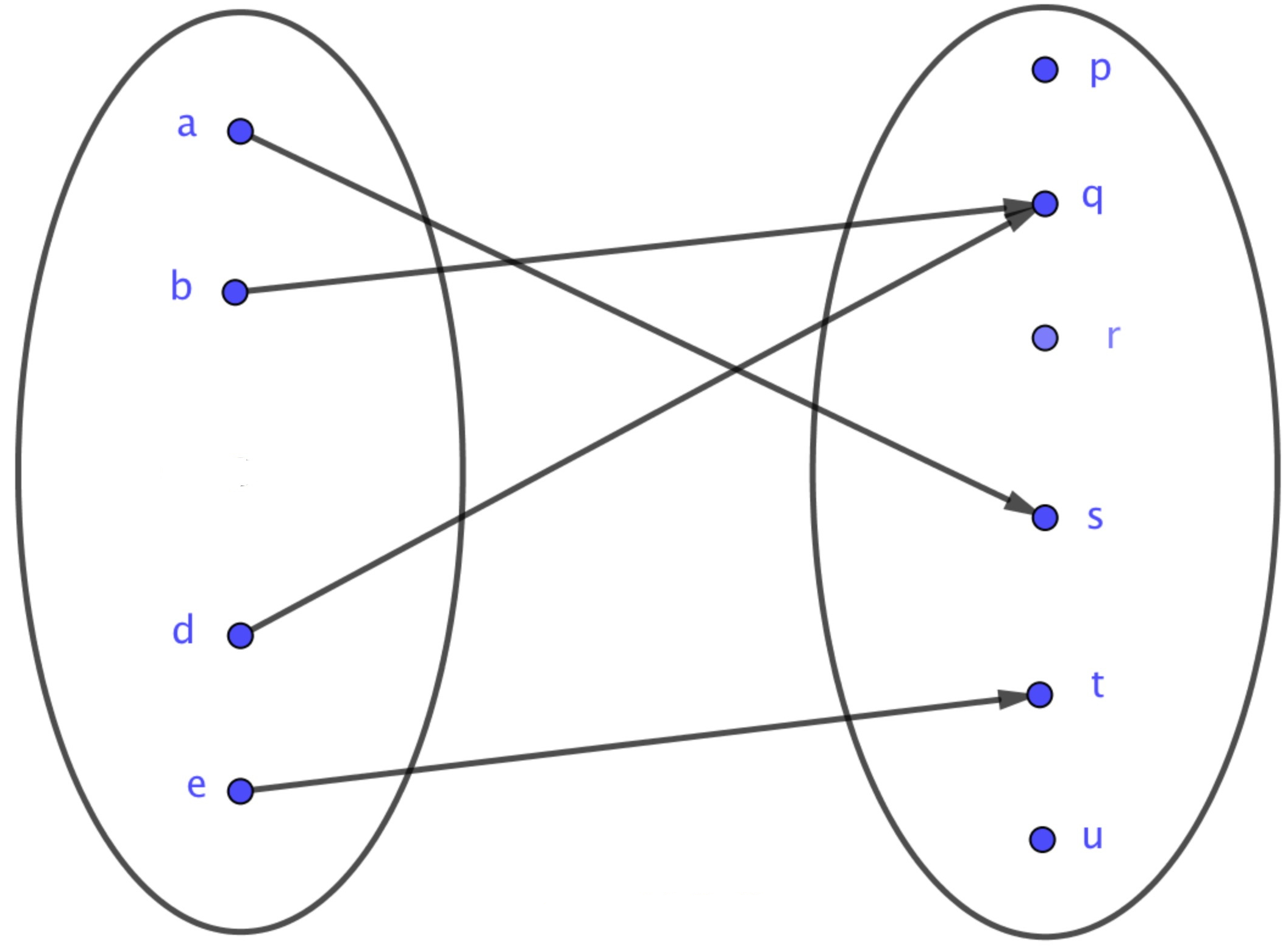
Définition d'une fonction
- Soit et deux ensembles. Une fonction de dans est la donnée d'une processus de correspondance qui à élément de permet d'associer élément de . Cet élément est alors noté . L'ensemble est alors appelé ensemble de départ et l'ensemble d'arrivée. Et il est d'usage d'adopter les écritures suivantes
ou encore
On dit que est l'image de par la correspondance .
On dit également que, s'il existe, que l'élément , tel que , est l'antécédent de par la correspondance .
On appelle de la fonction , noté , le sous-ensemble de qui contient tous les éléments qui admettent une image . Donc ; le cas implique que la fonction est alors une application.
Une fonction se représente par le diagramme sagittal suivant :Et dans ce cas, on a et . Ainsi on a .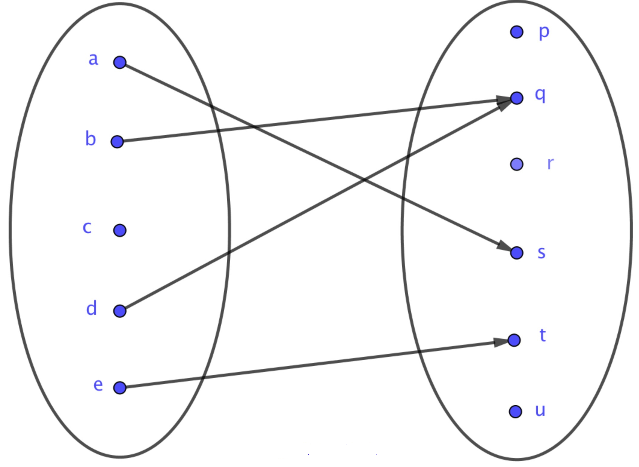
Pour bien comprendre la différence, illustrons ceci par un exemple simple donc pédagogique.
L'objet est une application et se représente par :
Une application se compose de trois éléments : l'ensemble de départ, l'ensemble d'arrivée et le processus de correspondance entre et . Si on change un de ces trois éléments, alors on change l'application et de fait on change ses propriétés. Illustrons ceci.
L'application se représente par :
Compositions des applications
- On considère les deux applications et suivantes :
et
Notons que l'ensemble d'arrivée de et le même que l'ensemble de départ de .
On commence par transformer par pour obtenir . Puis on transforme par pour obtenir .
On définit ainsi la composée par :
Et on a :
Et on associe la figure suivante :La composition des application . Si on considère les deux applications et , alors on a :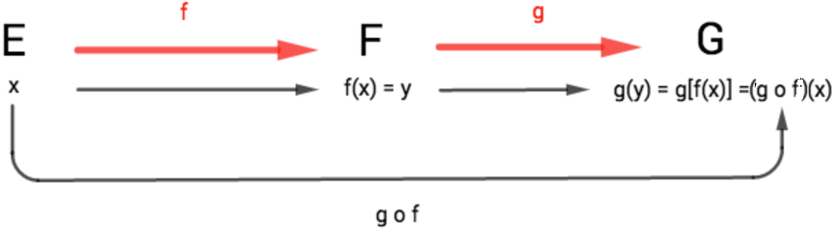
Par exemple. On considère les deux applications et suivantes :
et
Dans ce cas :
et
La composition des applications est une opération associative. Si , et sont trois applications, on a alors :
On définit sur l'ensemble , notée , par :
ou encore :
Soit et deux applications. On a alors :
et
Injections, surjections, bijections
Injection
- Soit une application. On dit que est une injection , ou que est injective, si tout élément de admet au plus un antécédent de .
Autrement dit, l'équation admet, au plus, une solution .
Ceci se traduit donc par l'assertion :
ou en prenant la contraposée :
Graphiquement, on a :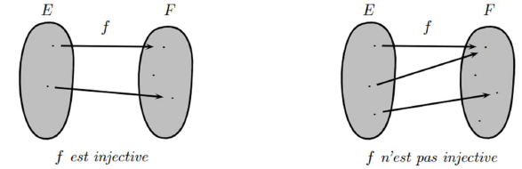
Par exemple, on considère l'application
Soit et deux nombres réels. On a :
Donc l'application est injective.
Pour une application de dans l'injectivité se traduit graphiquement par le fait que la droite horizontale à au plus un point d'intersection avec la représentation graphique de l'application considérée.
En outre, la composée de deux applications injectives est elle même injective.
Si est injective alors on peut affirmer que est injective.
Surjection
- Soit une application. On dit que est une surjection , ou que est surjective, si tout élément de admet au moins un antécédent de . On a alors .
Autrement dit, l'équation admet, au moins, une solution .
Ceci se traduit donc par l'assertion :
Graphiquement, on a :
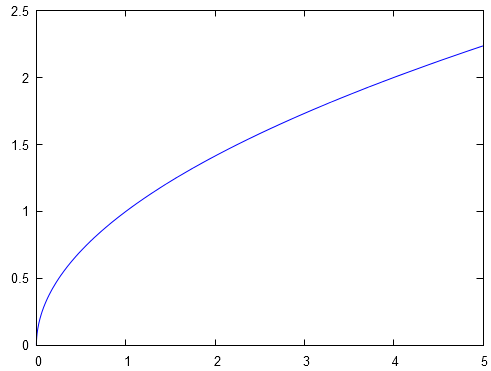
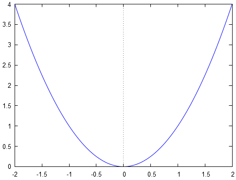
Par exemple, on considère l'application
Soit un nombre réel. On a :
Ainsi à chaque image il est possible d'associer au moins un antécédent : ou . Donc l'application est surjective.
Pour une application de dans la surjectivité se traduit graphiquement par le fait que la droite horizontale à au moins un point d'intersection avec la représentation graphique de l'application considérée.
En outre, la composée de deux applications surjectives est elle même surjective.
Si est surjective alors on peut affirmer que est surjective.
Bijection
- Soit une application. On dit que est une bijection , ou que est bijective, si tout élément de admet un unique antécédent de . On a alors .
Autrement dit, l'équation admet une unique solution .
Ceci se traduit donc par l'assertion :
Ce qui signifie qu'une application est bijective si elle est à la fois injective et surjective.
Graphiquement, on a :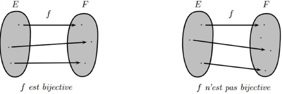
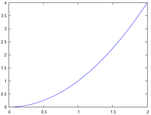
Par exemple, on considère l'application
Soit un nombre réel. On a :
Ainsi à chaque image il est possible d'associer un unique antécédent : .
Réciproquement, soit un antécédent, alors est l'unique image associée à l'antécédent . Donc l'application est bijective.
Considérons à nouveau l'application
Soit un nombre réel, et soit l'image de . On a :
Donc l'application est bijective. Ainsi cette application est également surjective. Nous avions démontrer précédemment qu'elle était injective.
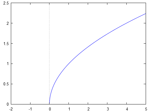
Pour une application de dans la bijectivité se traduit graphiquement par le fait que la droite horizontale à un unique point d'intersection avec la représentation graphique de l'application considérée.
Un théorème couramment utilisé est qu'une application de dans continue et strictement croissante réalise une bijection de sur son image par .
En outre, la composée de deux applications bijectives est elle même bijective.
Si est bijective alors on peut affirmer que est surjective et que est injective.
Soit un nombre réel. On a :
Ainsi à chaque image il est possible d'associer un unique antécédent : .
Réciproquement, soit un antécédent, alors est l'unique image associée à l'antécédent . Donc l'application est bijective.
Considérons à nouveau l'application
Soit un nombre réel, et soit l'image de . On a :
Donc l'application est bijective. Ainsi cette application est également surjective. Nous avions démontrer précédemment qu'elle était injective.
Pour une application de dans la bijectivité se traduit graphiquement par le fait que la droite horizontale à un unique point d'intersection avec la représentation graphique de l'application considérée.
Un théorème couramment utilisé est qu'une application de dans continue et strictement croissante réalise une bijection de sur son image par .
En outre, la composée de deux applications bijectives est elle même bijective.
Si est bijective alors on peut affirmer que est surjective et que est injective.
Bijections réciproques
Définition
- Soit une de dans . Comme est bijective, il est alors possible de construire une nouvelle et unique application de vers , qui à associe son unique antécédent. Cette application est appelée la de et se note ou . On a alors :
et
Avec :
Soit et deux applications bijectives. On note leur composée par :
Concernant la bijection réciproque de la composition , on a (attention à l'ordre) :
En effet, on a :
Puis :
En outre, la définition de la bijection réciproque permet d'écrire que :
On constate alors (par identification) que :
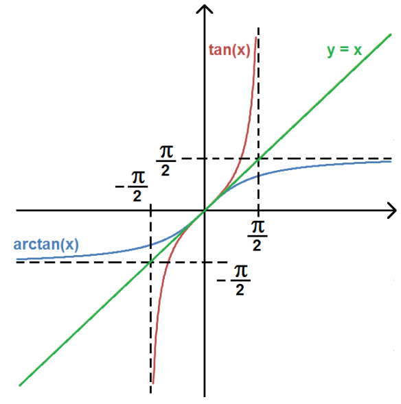
D'un point de vue graphique, les représentations graphiques des deux applications bijectives et , l'une par rapport à l'autre, par rapport à la droite d'équation (appelée première bissectrice du plan ).
Mentionnons quelques exemples classiques :
si alors . Donc .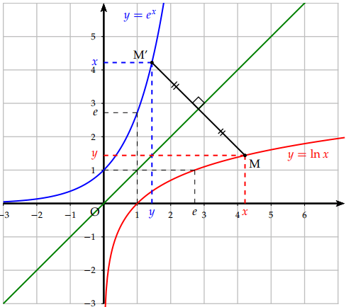 D'où :
Et :
Et :
si alors . Donc .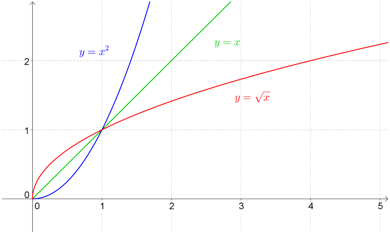 D'où :
Et :
Rappelons que :
Et :
Rappelons que :
si alors . Donc .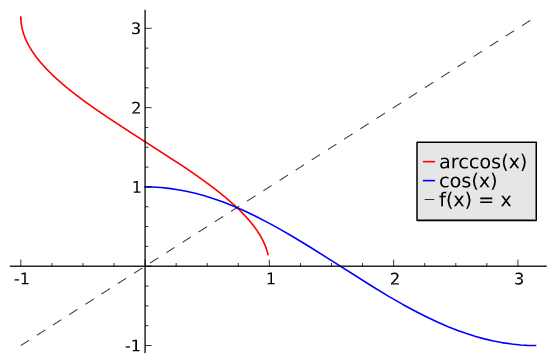 D'où :
Et :
Et :
si alors . Donc .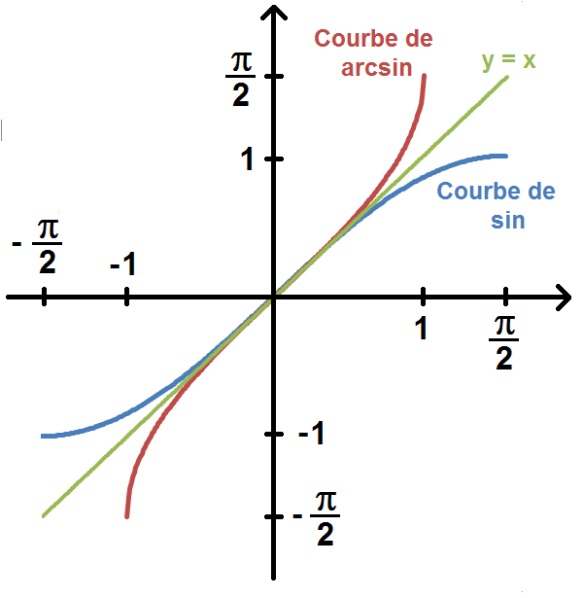 D'où :
Et :
Et :
si alors . Donc .
D'où :
Et :
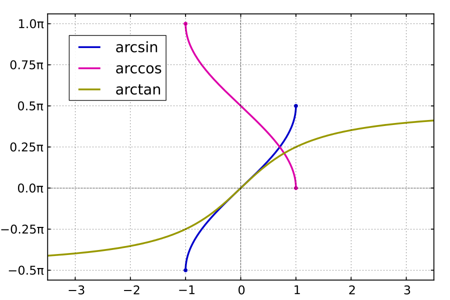
Il existe d'autres relations importantes qui croisent les applications trigonométriques et les applications trigonométriques réciproques. Citons les relations suivantes :
On prendra soin de conserver en mémoire l'allure des graphes des bijections réciproques trigonométriques (également très utilisées en Physique !) :
Signaler une erreur
Aide-nous à améliorer nos contenus en signalant les erreurs ou problèmes que tu penses avoir trouvés.