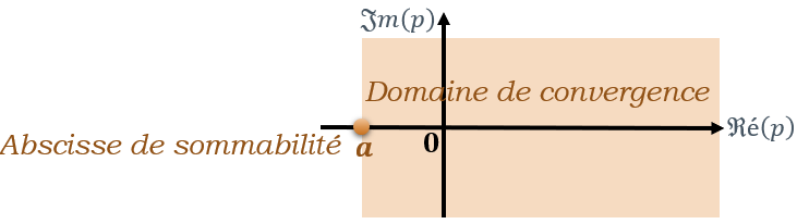
♣Deˊfinition Soit f une fonction numérique univariée de la variable x. Cette fonction f est supposée être nulle pour x<0. Une telle fonction est déclarée causale. On appelle Transformation de Laplace de f, la fonction notée F qui est définie, au travers du nombre complexe p, par l'intégrale généralisée suivante : F(p)=TLp[f(x)]=Lp[f(x)]=∫0+∞f(x)e−pxdx L'application TLp:f⟼F est appelée Transformation de Laplace de f et en langage opérationnel (ou symbolique) on note ceci comme F⊂f. De fait, la Transformation de Laplace n'existe que si l'intégrale généralisée ∫0+∞f(x)e−pxdx est convergente. On démontre mathématiquement que : - si f est continue par morceaux sur tout intervalle fermé [0;b] - si un nombre réel a existe, avec M>0, tel que, si à partir d'un certaine valeur particulière de x, notée x0, on a la majoration ∣f(x)∣⩽Meax alors F(p) est définie dans le demi-plan complexe ℜeˊ(p)>a. On a alors :
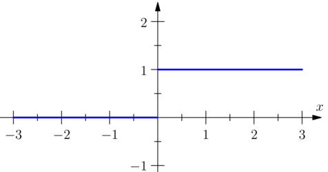
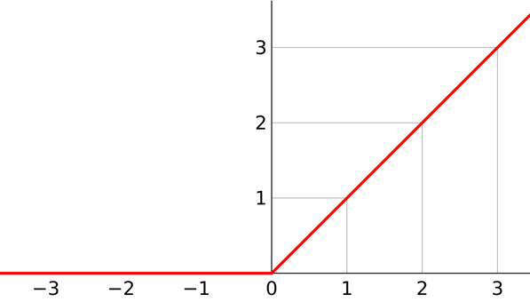
♣♣Transformeˊes usuelles ∙Fonction eˊchelon uniteˊ On a : U(x)=1 si x⩾0 et sinon U(x)=0. Soit :
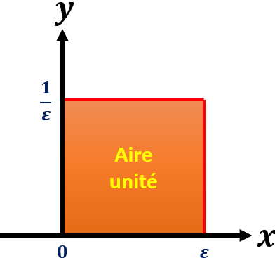
Dans ce cas, on a : F(p)=∫0+∞1e−pxdx=X⟶+∞lim[−pe−px]0X=X⟶+∞lim−pe−pX−e0=p1−X⟶+∞lime−pX Si ℜeˊ(p)>0 alors on a : X⟶+∞lim∣∣e−pX∣∣=X⟶+∞lime−ℜeˊ(p)X=0 Donc : TLp[U(x)]=F(p)=p1 avec ℜeˊ(p)>0. ∙∙Fonction impulsion uniteˊ ayant pour limite la distribution de Dirac Soit ε∈R+⋆. On considère la fonction porte Pε telle que : si x∈[0;ε[ alors Pε(x)=1 sinon Pε(x)=0 :
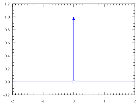
On constate immédiatement que : ∫−∞+∞Pε(x)dx=1 On appelle distribution de Dirac, notée δ(x), la limite de Pε lorsque ε⟶0 : δ(x)=ε⟶0limPε(x) La distribution de Dirac sert à positionner une action, soit en temps soit en position. Graphiquement, cet objet mathématique se représente comme :
On a : TLp[Pε(x)]=∫0+∞Pε(x)e−pxdx=∫0εε1e−pxdx=ε1∫0εe−pxdx=ε1[−pe−px]0ε=pε1[−e−px]0ε=pε1[e−px]ε0 D'où : TLp[Pε(x)]=pε1(e−p0−e−pε)=pε1(1−e−pε) Passons à la limite lorsque ε⟶0. On a alors : e−pε0∼1−pε Donc on obtient : TLp[δ(x)]=ε⟶0limTLp[Pε(x)]=ε⟶0lim(pε1(1−e−pε))0∼ε⟶0lim(pε1(1−1+pε)) Finalement, on trouve que : TLp[δ(x)]=1. ∙∙∙Fonction rampe On a : R(x)=x si x⩾0 et sinon R(x)=0. On peut également écrire que R(x)=xU(x). Soit :
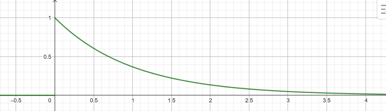
Dans ce cas, on a : TLp[R(x)]=F(p)=∫0+∞xe−pxdx On va faire usage d'une intégration par parties. On a alors : TLp[R(x)]=F(p)=[x×−pe−px]0+∞−∫0+∞1×−pe−pxdx Soit : TLp[R(x)]=F(p)=−p1[xe−px]0+∞+p1∫0+∞e−pxdx=−p1x⟶+∞lim(xe−px)+p1∫0+∞e−pxdx Soit encore : TLp[R(x)]=F(p)=−p1x⟶+∞lim(xe−px)+p1∫0+∞U(x)e−pxdx=−p1x⟶+∞lim(xe−px)+p1TLp[U(x)] Ainsi : TLp[R(x)]=F(p)=−p1x⟶+∞lim(xe−px)+p1p1=−p1x⟶+∞lim(xe−px)+p21 Si ℜeˊ(p)>0 alors on a : x⟶+∞limxe−px=0 Finalement : TLp[R(x)]=p21(ℜeˊ(p)>0) De manière similaire, on démontre que : TLp[xnU(x)]=pn+1n!(ℜeˊ(p)>0;n∈N) ∙∙∙∙Fonctions exponentielles Soit a⩾0. On a : E(x)=e−ax si x⩾0 et sinon E(x)=0. On peut également écrire que E(x)=e−axU(x). Soit, par exemple :
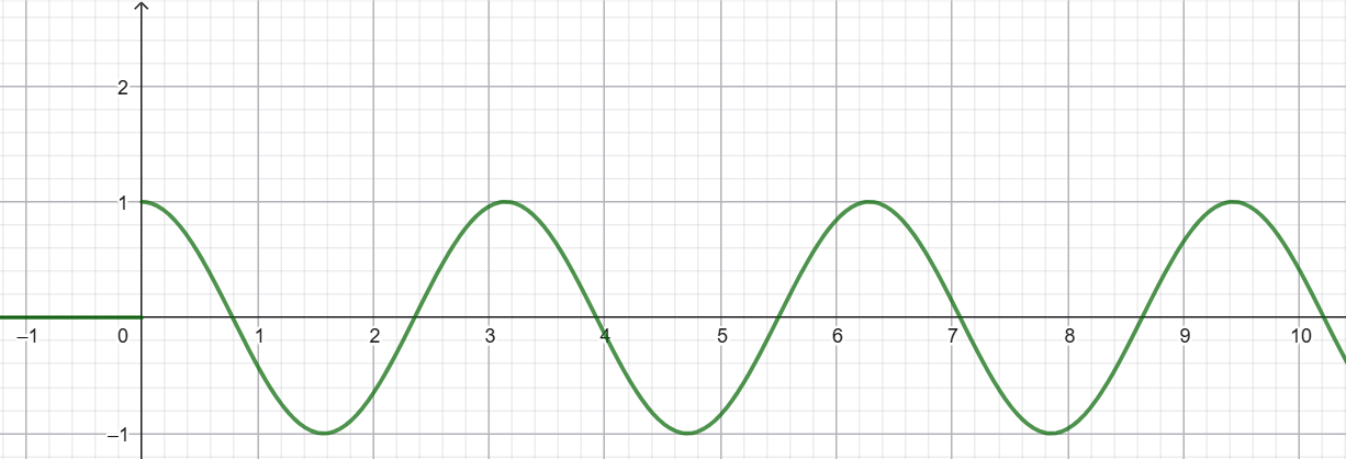
Dans ce cas, on a : TLp[E(x)]=F(p)=∫0+∞e−axe−pxdx=∫0+∞e−(p+a)xdx=X⟶+∞lim[−(p+a)e−(p+a)x]0X=p+a1X⟶+∞lim[e−(p+a)x]X0 Soit : Dans ce cas, on a : TLp[E(x)]=F(p)=p+a1(e−a0−X⟶+∞lime−(p+a)X)=p+a1(1−X⟶+∞lime−(p+a)X) Si ℜeˊ(p)>0 alors on a : X⟶+∞lim∣∣e−(p+a)X∣∣=X⟶+∞lime−(ℜeˊ(p)+a)X=0 Donc : TLp[E(x)]=TLp[e−axU(x)]=p+a1(ℜeˊ(p)>0) ∙∙∙∙∙Fonction cosinus Soit i le nombre complexe imaginaire tel que i2=−1. Soit ω⩾0. On a : C(x)=cos(ωx) si x⩾0 et sinon C(x)=0. On peut également écrire que C(x)=cos(ωx)U(x). Soit, par exemple :
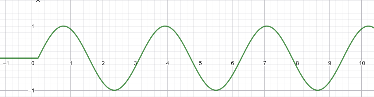
On a donc : TLp[C(x)]=TLp[cos(ωx)] En faisant usage des formules d'Euler, on peut alors écrire que : TLp[C(x)]=TLp[2eiωx+e−iωx]=21TLp[eiωx+e−iωx]=21TLp[eiωxU(x)+e−iωxU(x)] Par linéarité de l'intégrale, on a alors : TLp[C(x)]=21(TLp[eiωxU(x)]+TLp[e−iωxU(x)]) En utilisant le résultat précédent relatif aux fonctions exponentielles, on a alors : TLp[C(x)]=21(p−iω1+p+iω1)=21((p−iω)×(p+iω)p+iω+p−iω)=21×p2+ω22p Finalement : TLp[C(x)]=TLp[cos(ωx)U(x)]=p2+ω2p(ℜeˊ(p)>0) ∙∙∙∙∙∙Fonction sinus Soit i le nombre complexe imaginaire tel que i2=−1. Soit ω⩾0. On a : S(x)=sin(ωx) si x⩾0 et sinon S(x)=0. On peut également écrire que S(x)=sin(ωx)U(x). Soit, par exemple :
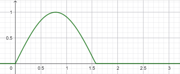
On a donc : TLp[S(x)]=TLp[sin(ωx)] En faisant usage des formules d'Euler, on peut alors écrire que : TLp[S(x)]=TLp[2ieiωx−e−iωx]=2i1TLp[eiωx−e−iωx]=2i1TLp[eiωxU(x)−e−iωxU(x)] Par linéarité de l'intégrale, on a alors : TLp[S(x)]=2i1(TLp[eiωxU(x)]−TLp[e−iωxU(x)]) En utilisant le résultat précédent relatif aux fonctions exponentielles, on a alors : TLp[S(x)]=2i1(p−iω1−p+iω1)=2i1((p−iω)×(p+iω)p+iω−p+iω)=2i1×p2+ω22iω Finalement, en simplifiant par 2i, on obtient : TLp[S(x)]=TLp[sin(ωx)U(x)]=p2+ω2ω(ℜeˊ(p)>0) ♣♣♣Proprieˊteˊs de la transformation de Laplace ∙La lineˊariteˊ Soit a et b deux nombres réels.Soient f et g deux fonctions numériques univariées intégrables. On a alors : TLp[a×f(x)+b×g(x)]=a×TLp[f(x)]+b×TLp[g(x)] Par exemple : TLp[sin2(ωx)U(x)]=TLp[21−cos(2ωx)U(x)]=21×TLp[U(x)]−21×TLp[cos(2ωx)U(x)] D'après tout ce qui précède, on a alors : TLp[sin2(ωx)U(x)]=21×p1−21×p2+(2ω)2p En ordonnant les termes, on obtient : TLp[sin2(ωx)U(x)]=2p1(1−p2+4ω2p2)=2p1(p2+4ω2p2+4ω2−p2+4ω2p2)=2p1(p2+4ω2p2+4ω2−p2) Soit : TLp[sin2(ωx)U(x)]=2p1(p2+4ω24ω2) Finalement : TLp[sin2(ωx)U(x)]=p(p2+4ω2)2ω2 ∙∙Le deˊcallage Soit a un nombre réel strictement positif. Soit f une fonction numérique univariée intégrable et causale. On pose alors : g(x)=f(x−a) si x⩾a sinon g(x)=0. On a alors : TLp[g(x)]=∫0+∞g(x)e−pxdx=∫0+∞f(x−a)e−pxdx Posons X=x−a. Dans ce cas on a x=X+a et dx=dX. D'où : TLp[g(x)]=∫−a+∞f(X)e−p(X+a)dX=∫−a0f(X)e−p(X+a)dX+∫0+∞f(X)e−p(X+a)dX Comme f est causale, on a immédiatement : TLp[g(x)]=0+∫0+∞f(X)e−p(X+a)dX=∫0+∞f(X)e−pXe−padX=e−pa∫0+∞f(X)e−pXdX=e−pa×TLp[f(x)] Finalement, avec a>0, on a : TLp[f(x−a)U(x−a)]=e−pa×TLp[f(x)] Ce résultat est connu sous le nom de theˊoreˋme du retard. Par exemple, on considère la fonction suivante : f(x)=sin(2x) si 0⩽x⩽2π sinon f(x)=0. Graphiquement, on a :
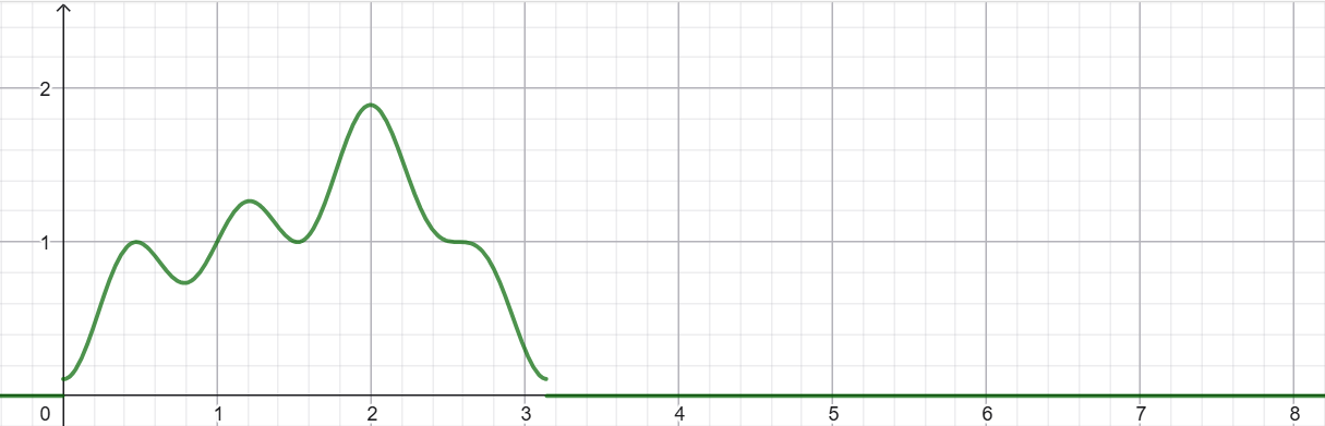
Cette fonction peut encore s'écrire à l'aide de la fonction échelon U. En effet, on a : f(x)=sin(2x)U(x)+sin(2(x−2π))U(x−2π) La seconde partie sert à annuler le reste présent apreˋs le premier lobe par un simple décalage de 2π car : ∀x∈R,sin(2(x−2π))=sin(2x−π)=−sin(2x). Ainsi, on peut écrire que : TLp[f(x)]=TLp[sin(2x)U(x)+sin(2(x−2π))U(x−2π)] Soit : TLp[f(x)]=TLp[sin(2x)U(x)]+TLp[sin(2(x−2π))U(x−2π)] Soit encore : TLp[f(x)]=p2+222+e−p2π×p2+222 Finalement : TLp[f(x)]=p2+42(1+e−p2π) ∙∙∙Cas des fonctions peˊriodiques Soit T un nombre réel strictement positif. Soit f une fonction numérique univariée intégrable, T-périodique et causale. Le motif élémentaire est représenté par la fonction motif fm suivante, qui peut-être, sur l'intervalle [0;T], représentée par :
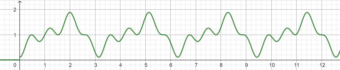
Donc f aurait pour représentation graphique suivante :
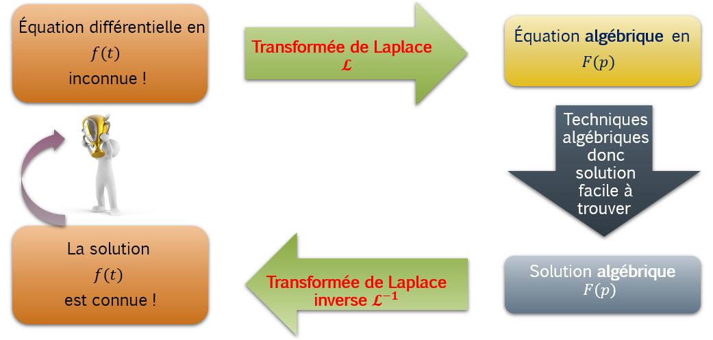
Donc la fonction f va pouvoir s'écrire comme une somme de fonction motif mais décalées les uns par par rapport aux autre de T. Donc : f(x)=fm(x)+fm(x−T)+fm(x−2T)+fm(x−3T)+⋯ Soit : f(x)=n=0∑+∞fm(x−nT) En introduisant la transformation de Laplace, on a alors par linéarité de cette dernière : TLp[f(x)]=TLp[n=0∑+∞fm(x−nT)]=n=0∑+∞TLp[fm(x−nT)] Le théorème du retard nous permet alors d'écrire que : TLp[f(x)]=n=0∑+∞epnT×TLp[fm(x)] Le terme TLp[fm(x)] est indépendant de n donc il peut sortir de la sommation. On obtient alors : TLp[f(x)]=TLp[fm(x)]×n=0∑+∞e−pnT De plus, on a : n=0∑+∞e−pnT=n=0∑+∞(e−pT)n=1+e−pT+(e−pT)2+(e−pT)3+⋯ En supposant que ∣e−pT∣<1, ce qui revient à avoir ℜeˊ(p)>0, on obtient une sommation de série géométrique de raison e−pT. Donc on obtient : n=0∑+∞e−pnT=1−e−pT1 On obtient finalement : TLp[f(x)]=TLp[fm(x)]×1−e−pT1 Par exemple, on considère la fonction créneau causale f qui est 2-périodique et qui s'exprime au travers de son motif fm comme : fm(x)=1 si 0⩽x<1 et fm(x)=−1 si 1⩽x<2. On peut écrire cela de la manière suivante : fm(x)=U(x)+U(x−2)−2U(x−1) Ainsi, la transformation de Laplace de la fonction motif est : TLp[fm(x)]=p1+e−p2p1−2e−p1p1=p1(1+e−2p−2e−p)=p1(1+(e−p)2−2e−p) Donc : TLp[fm(x)]=p1(1−2e−p+(e−p)2)=p1(1−e−p)2 On obtient alors, avec le théorème des fonctions périodiques : TLp[f(x)]=p1(1−e−p)2×1−e−p21=p1(1−e−p)2×12−(e−p)21=p1(1−e−p)2×(1+e−p)×(1−e−p)1 En simplifiant par le terme 1−e−p on obtient finalement : TLp[f(x)]=p1×1+e−p1−e−p ∙∙∙∙Transformeˊe de Laplace de la deˊriveˊe d’une fonction On considère une fonction numérique univariée f causale et qui est dérivable sur R+. La fonction dérivée, notée f′ est continue par morceaux sur tout intervalle fermés de R+. On a alors : TLp[f′(x)]=∫0+∞f′(x)e−pxdx A l'aide d'une intégration par parties, on obtient : TLp[f′(x)]=[f(x)e−px]0+∞−∫0+∞f(x)(−p)e−pxdx Soit : TLp[f′(x)]=X⟶+∞lim[f(x)e−px]0X+p∫0+∞f(x)e−pxdx Soit encore : TLp[f′(x)]=X⟶+∞lim(f(X)e−pX)−f(0)e−p0+p∫0+∞f(x)e−pxdx Ce qui nous donne donc : TLp[f′(x)]=X⟶+∞lim(f(X)e−pX)−f(0)+pF(p) Or, il existe un nombre réel a, avec M>0, tel qu'à partir d'un certaine valeur particulière X0, on a la majoration ∣f(X)∣⩽MeaX. Donc : ∣f(X)e−pXC∣⩽MeaXe−ℜeˊ(p)X=Me−(ℜeˊ(p)−a)X Ainsi, si ℜeˊ(p)>a on a X⟶+∞lim(f(X)e−pX)=0. Finalement : TLp[f′(x)]=pF(p)−f(0) ∙∙∙∙∙Transformeˊe de Laplace de la deˊriveˊe seconde d’une fonction De la même manière, on a : TLp[f′′(x)]=pTLp[f′(x)]−f′(0)=p(pF(p)−f(0))−f′(0)=p2F(p)−pf(0)−f′(0) Soit : TLp[f′′(x)]=p2F(p)−pf(0)−f′(0) ∙∙∙∙∙∙Transformeˊe de Laplace de la deˊriveˊe troisieˋme d’une fonction De la même manière, on a : TLp[f′′′(x)]=pTLp[f′′(x)]−f′′(0)=p(p2F(p)−pf(0)−f′(0))−f′′(0)=p3F(p)−p2f(0)−pf′(0)−f′′(0) Soit : TLp[f′′(x)]=p3F(p)−p2f(0)−pf′(0)−f′′(0) ∙∙∙∙∙∙∙Theˊoreˋme de la valeur finale et initiale On a vu que : TLp[f′(x)]=∫0+∞f′(x)e−pxdx=pF(p)−f(0) Or, on sait que : p⟶+∞lim(f′(x)e−px)=0 Donc : p⟶+∞limTLp[f′(x)]=0 D'où la relation suivante : p⟶+∞limpF(p)=f(0) Cette dernière relation s'appelle le théorème de la valeur initiale. De plus, on a donc : ∫0+∞f′(x)e−pxdx=pF(p)−f(0) Faisons tendre p vers 0. On a alors p⟶0lime−px=1 On a alors : p⟶0lim∫0+∞f′(x)e−pxdx=∫0+∞f′(x)dx=[f(x)]0+∞=b⟶+∞lim[f(x)]0b=b⟶+∞limf(b)−f(0) On peut donc écrire que : p⟶0lim∫0+∞f′(x)e−pxdx=p⟶0lim(pF(p)−f(0))=p⟶0lim(pF(p))−f(0) D'où l'égalité suivante : p⟶0lim(pF(p))−f(0)=b⟶+∞limf(b)−f(0) En simplifiant : p⟶0lim(pF(p))=b⟶+∞limf(b) Finalement, comme b est une notation muette, nous pouvons écrire que : p⟶0lim(pF(p))=x⟶+∞limf(x) Cette dernière relation s'appelle le théorème de la valeur finale. ∙∙∙∙∙∙∙∙Transformeˊe de la primitive On pose ψ(x)=∫0xf(x)dx. Ceci implique que ψ′(x)=f(x) et que ψ(x=0)=0. Donc on a : TLp[ψ′(x)]=pTLp[ψ(x)]−ψ(0)=pTLp[ψ(x)]−0=pTLp[ψ(x)] Ceci vas donc s'écrire comme : TLp[f(x)]=pTLp[∫0xf(x)dx] Finalement : [∫0xf(x)dx]=pTLp[f(x)]⟺[∫0xf(x)dx]=pF(p) ♣♣♣♣Application aux eˊquations diffeˊrentielles Les propriétés précédentes permettent de transformer une équation différentielle linéaire en une équation algébrique. Le mécanisme est le suivante :
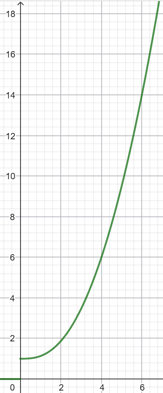
Pour illustrer la méthode, nous allons considérer le problème de Cauchy simple suivant : f′′(x)+f′(x)=x(x⩾0) Avec les deux conditions initiales suivantes : f(x=0)=1 et f′(x=0)=0 Commençons par prendre la transformée de Laplace des deux membres de l'équations différentielle ordinaire (EDO) considérée : TLp[f′′(x)+f′(x)]=TLp[x] Par linéarité, on a alors : TLp[f′′(x)]+TLp[f′(x)]=TLp[x] Si on adopte la notation usuelle TLp[f(x)]=F(p) alors on a : * TLp[f′′(x)]=p2F(p)−pf(0)−f′(0)=p2F(p)−p1−0=p2F(p)−p ** TLp[f′(x)]=pF(p)−f(0)=pF(p)−1 Donc : p2F(p)−p+pF(p)−1=TLp[x] D'après les débuts de ces rappels de cours, on sait que la transformée de laplace de la fonction rampe est : TLp[R(x)]=TLp[x]=p21. Donc, on obtient : p2F(p)−p+pF(p)−1=p21⟺p2F(p)+pF(p)=1+p+p21⟺(p2+p)F(p)=1+p+p21 Soit : p(p+1)F(p)=1+p+p21 Soit encore : F(p)=p(p+1)1+p(p+1)p+p3(p+1)1 En simplifiant : F(p)=p(p+1)1+p+11+p3(p+1)1 D'après les tables de correspondances, on a : p(p+1)1=TLp[1−e−x] et p+11=TLp[e−x] De plus, on peut faire une décomposition en éléments simples du terme p3(p+1)1. On a alors : p3(p+1)1=pA+p2B+p3C+p+1Davec(A;B;C;D)∈R4 Donc : p31=App+1+Bp2p+1+Cp3p+1+D Si on pose p=−1 alors on a : (−1)31=A−1−1+1+B(−1)2−1+1+C(−1)3−1+1+D⟺−1=D Puis, on a p+11=App3+Bp2p3+C−p+1p3 Soit : p+11=Ap2+Bp+C−p+1p3 Si on pose p=0 alors on a : 0+11=A02+B0+C−0+103⟺1=C Donc on a : p3(p+1)1=pA+p2B+p31−p+11 Posons p=1 on a alors : 13(1+1)1=1A+12B+131−1+11⟺21=A+B+1−21⟺21=A+B+21⟺0=A+B Donc B=−A. Ainsi : p3(p+1)1=pA−p2A+p31−p+11 Posons p=2 on a alors : 23(2+1)1=2A−22A+231−2+11⟺241=2A−4A+81−31⟺241=4A−245⟺1=6A−5 Donc 6=6A et de fait A=1 ce qui implique que B=−1. Ceci nous permet d'écrire que : p3(p+1)1=p1−p21+p31−p+11 Ainsi par linéarité et d'après les débuts de nos rappels de cours, et comme x⩾0, on a : TLp[p3(p+1)1]=TLp[1]−TLp[x]+TLp[2x2]−TLp[e−x] D'où : TLp[p3(p+1)1]=TLp[1−x+2x2−e−x] De fait : F(p)=TLp[1−e−x]+TLp[e−x]+TLp[1−x+2x2−e−x] Soit : TLp[f(x)]=TLp[1−e−x+e−x+1−x+2x2−e−x] En simplifiant : TLp[f(x)]=TLp[2−x+2x2−e−x] Ainsi, on en déduit que : f(x)=2−x+2x2−e−x=21(x2−2x+4)−e−x Cependant, on sait que −e−x=sinh(x)−cosh(x). Ceci nous permet également d'avoir : f(x)=21(x2−2x+4)+sinh(x)−cosh(x)avec:x⩾0 Ou alors on fait intervenir l'échelon unité pour se passer de la condition x⩾0. On a alors : f(x)=(21(x2−2x+4)+sinh(x)−cosh(x))U(x) Graphiquement on obtient :
♣♣♣♣♣La transformation de Laplace inverse ∙Deˊfinition Lorsque l'on note F(p)=TLp[f(x)]=Lp[f(x)] dans ce cas, on dit que f est l’original de F. On note cela comme : f(x)=TLx−1[F(p)]=Lx−1[F(p)] Du point vue fonctionnelle, avec i2=−1, on a : f(x)=2πi1∫ChemindansleplancomplexeF(p)epxdp Cette formule est connue sous le nom de transformation de Bromwich. Son usage est technique et sort totalement du contexte de ces rappels de cours. C'est pourquoi il est d'usage de faire emploi de tables de correspondances. Un telle table vous sera donnée à la fin de ces rappels de cours. Nous pouvons mentionner que la transformation de Laplace inverse est linéaire et qu'elle exigera les mêmes réflexes que la transformation de Laplace. ∙∙Exemple Recherchons l'original de F(p)=(p2+ω2)(p2+Ω2)1 ou ω et Ω sont deux nombres réels distincts. Pour faire cela, nous allons effectuer une décomposition en éléments simples. Avec les quatre nombres réels A, B, C et D on a : F(p)=(p2+ω2)(p2+Ω2)1=p2+ω2Ap+B+p2+Ω2Cp+D On remarque que, par rapport à p, l'expression F(p)=(p2+ω2)(p2+Ω2)1 est paire. Ceci implique immédiatement que l'expression p2+ω2Ap+B+p2+Ω2Cp+D doit également l'être. De fait A=C=0. Puis, posons p=0. On a alors : (02+ω2)(02+Ω2)1=02+ω2B+02+Ω2D⟺ω2Ω21=ω2B+Ω2D⟺ω2Ω21=ω2Ω2BΩ2+Dω2 Soit BΩ2+Dω2=1. On a alors :: B=Ω21−Dω2 De plus, nous avions : (p2+ω2)(p2+Ω2)1=p2+ω2B+p2+Ω2D⟹p2+ω21=Bp2+ω2p2+Ω2+D Posons alors p2=−Ω2 et nous obtenons : −Ω2+ω21=Bp2+ω2−Ω2+Ω2+D⟺ω2−Ω21=D⟺−Ω2−ω21=D De fait, on a alors : B=Ω21−Dω2=Ω21−(−Ω2−ω21)ω2=Ω21+Ω2−ω2ω2=Ω2Ω2−ω2Ω2−ω2+Ω2−ω2ω2=Ω2Ω2−ω2Ω2−ω2+ω2=Ω2Ω2−ω2Ω2 En simplifiant par Ω2 on trouve que B=−D=Ω2−ω21.De fait, on trouve que : (p2+ω2)(p2+Ω2)1=Ω2−ω21p2+ω21−Ω2−ω21p2+Ω21=Ω2−ω21(p2+ω21−p2+Ω21) Donc, nous pouvons écrire que: F(p)=Ω2−ω21(ω1p2+ω2ω−Ω1p2+Ω2Ω) Prenons la transformation inverse de Laplace de cette équation. On a alors : TLx−1[F(p)]=TLx−1[Ω2−ω21(ω1p2+ω2ω−Ω1p2+Ω2Ω)] Par linéarité, nous avons donc : TLx−1[F(p)]=Ω2−ω21(ω1TLx−1[p2+ω2ω]−Ω1TLx−1[p2+Ω2Ω]) D'où : f(x)=Ω2−ω21(ω1sin(ωx)−Ω1sin(Ωx)) On peut faire apparaitre un sinus cardinal selon : f(x)=Ω2−ω2x(sinc(ωx)−sinc(Ωx)) ∙∙∙L’original de F(p+a) Soit f(x)=TLx−1[F(p)]. On a : F(p+a)=∫0+∞f(x)e−(p+a)xdx=∫0+∞f(x)e−axe−pxdx=∫0+∞(f(x)e−ax)e−pxdx Finalement : TLx−1[F(p+a)]=f(x)e−ax Ou de même : TLp[f(x)e−ax]=F(p+a) Par exemple, on a : TLp[e−axcos(ωx)]=(p+a)2+ω2p+a Mais aussi : TLp[e−axsin(ωx)]=(p+a)2+ω2ω Par exemple, recherchons l'original de l'expression F(p)=p2+p+1p. Si l'on effectue une mise sous forme canonique, on obtient alors : F(p)=p2+p+1p=(p+21)2+43p Et on a alors les jeux d'écritures suivants : F(p)=(p+21)2+43p=(p+21)2+43p+21−21=(p+21)2+43p+21−(p+21)2+4321 Que nous allons écrire comme : F(p)=(p+21)2+(23)2p+21−21(p+21)2+(23)21 Soit : TLx−1[F(p)]=TLx−1⎣⎡(p+21)2+(23)2p+21−21(p+21)2+(23)21⎦⎤ Soit encore par linéarité : TLx−1[F(p)]=TLx−1⎣⎡(p+21)2+(23)2p+21⎦⎤−21TLx−1⎣⎡(p+21)2+(23)21⎦⎤ On a également : TLx−1[F(p)]=TLx−1⎣⎡(p+21)2+(23)2p+21⎦⎤−21231TLx−1⎣⎡(p+21)2+(23)223⎦⎤ D'après ce qui précède, nous en déduisons immédiatement que : f(x)=e−21xcos(23x)−31e−21xsin(23x) En factorisant, on obtient : f(x)=3e−21x(3cos(23x)−sin(23x)) Finalement, en introduisant l'échelon unité afin de rendre la fonction f causale, on trouve que : f(x)=3e−21x(3cos(23x)−sin(23x))U(t) ∙∙∙∙L’original de F′(p) On admettra, sans démonstration que : TLx−1[F′(p)]=−xf(x) Par exemple, on sait que : TLp[sin(ωx)]=p2+ω2ω Or, on a : (p2+ω2ω)′=(p2+ω2)2−(p2+ω2)′ω=(p2+ω2)2−2pω Donc, d'après le résultat admis juste ci-avant, on a : TLx−1[(p2+ω2)2−2pω]=−xsin(ωx) Finalement, on a : TLx−1[(p2+ω2)22pω]=xsin(ωx) Identiquement : TLp[xsin(ωx)]=(p2+ω2)22pω ∙∙∙∙∙L’original de ∫p+∞F(u)du On admettra, sans démonstration que : TLx−1[∫p+∞F(u)du]=xf(x) ♣♣♣♣♣♣L’original du produit de deux transformeˊes de Laplace ∙Le produit de convolution de deux fonctions causales On considère les deux fonctions causales f et g. Le produit de convolution des deux fonctions f et g est noté f⋆g et est défini par : (f⋆g)(x)=∫0xf(t)×g(x−t)dt On rappelle que (f⋆g)(x)=(g⋆f)(x). ∙∙Le produit de convolution et la transformation de Laplace On considère les deux fonctions causales f et g. On note F(p)=TLp[f(x)] et G(p)=TLp[g(x)]. On a alors le résultat suivant : TLx−1[F(p)×G(p)]=(f⋆g)(x) Ce qui implique que : TLp[(f⋆g)(x)]=F(p)×G(p) En effet, on a : TLp[(f⋆g)(x)]=TLp[∫0xf(t)×g(x−t)dt] Soit : TLp[(f⋆g)(x)]=∫0+∞∫0xf(t)×g(x−t)dte−pxdx Posons v=x−t. Dans ce cas, on a x=v+t et dxdv=dxd(x−t)=1 donc dx=dv. De plus, la borne x peut-être étendue à l'infini puisque dans la définition de la transformée de Laplace x va jusqu'à l'infini lors du processus d'intégration. On a alors : TLp[(f⋆g)(x)]=∫0+∞∫0+∞f(t)×g(v)dte−p(t+v)dv Soit : TLp[(f⋆g)(x)]=∫0+∞∫0+∞f(t)×g(v)dte−pte−pvdv Soit encore : TLp[(f⋆g)(x)]=∫0+∞∫0+∞f(t)e−ptdt×g(v)e−pvdv Ce qui nous donne donc : TLp[(f⋆g)(x)]=∫0+∞f(t)e−ptdt×∫0+∞g(v)e−pvdv Comme une variable d'intégration est une variable muette, on obtient donc le résultat annoncé ci-avant, à savoir que l'on a : TLp[(f⋆g)(x)]=∫0+∞f(t)e−pxdx×∫0+∞g(x)e−pxdx Finalement : TLp[(f⋆g)(x)]=F(p)×G(p) ♣♣♣♣♣♣♣Table partielle Soit n∈N⋆. Les nombres a, b, c et d sont des nombres réels. La constante d'Euler-Mascheroni est notée γ. Nous considérerons des fonctions numériques univariées f causales. Pour nous, la distribution de Dirac sera notée δ. Pour nous, la fonction Gamma d'Euler sera notée Γ. Pour nous, la première des fonctions de Bessel de première espèce sera notée J0. Nous désignerons par erf la fonction d’erreur de Gauss : erf(x)=π2∫0xe−t2dt Nous désignerons par erfc la fonction d’erreur complémentaire de Gauss : erfc(x)=1−erf(x)=π2∫x+∞e−t2dt Nous désignerons par Si la fonction Sinus intégral de Fresnel : Si(x)=∫0xtsin(t)dt On a les correspondances suivantes qui sont très pratiques dans les usages de la transformation de Laplace : f(x)↭F(p) 0↭0 δ(x)↭1 1↭p1 x↭p21 x2↭p32 x3↭p46 xn↭pn+1n! mais également pn+1Γ(n+1) x↭21p3π x1↭pπ e−ax↭p+a1 xe−ax↭(p+a)21 x2e−ax↭(p+a)32 xne−ax↭(p+a)n+1n! mais également (p+a)n+1Γ(n+1) a1(1−e−ax)↭p(p+a)1 a21(e−ax+ax−1)↭p2(p+a)1 a31(a2x2−ax+1−e−ax)↭p3(p+a)1 a21−(1+ax)e−ax↭p(p+a)21 2a3e−ax(2eax−a2x2−2ax−2)↭p(p+a)31 2a4e−ax(2axeax−6eax+a2x2+4ax+6)↭p2(p+a)31 2a3sin(ax)−axcos(ax)↭(p2+a2)21 a−be−bx−e−ax↭(p+a)(p+b)1 a−bae−ax−be−xb↭(p+a)(p+b)p (a−b)(a−c)(b−c)(b−c)e−ax+(c−a)e−bx+(a−b)e−cx↭(p+a)(p+b)(p+c)1 (a−b)2e−ax((a−b)x−1)+e−bx↭(p+a)(p+b)21 ab(a−b)(c−a)be−ax+(b−c)ae−bx+(a−b)c↭p(p+a)(p+b)p+c ab(a−b)(a2−ac+d)be−ax−(b2−bc+d)ae−bx+(a−b)d↭p(p+a)(p+b)p2+cp+d ax↭p−ln(a)1 xe−bx−e−ax↭ln(p+bp+a) ln(x)↭−pln(p)+γ xln(x)↭126ln(p)(ln(p)+2γ)+π2+6γ2 x2(1−cos(ax))↭ln(p2p2+a2) x2(1−cosh(ax))↭ln(p2p2−a2) sin(ax)↭p2+a2a xsin(ax)↭arctan(pa) sinc(ax)↭a1arctan(pa) cos(ax)↭p2+a2p xsin(ax)↭(p2+a2)22ap xcos(ax)↭(p2+a2)2p2−a2 x2sin(ax)↭(p2+a2)32a(3p2−a2) x2cos(ax)↭(p2+a2)32p(p2−3a2) x3sin(ax)↭(p2+a2)424ap(p2−a2) x3cos(ax)↭(p2+a2)46(p4−6a2p2+a4) sin(ax+b)↭p2+a2acos(b)+psin(b) cos(ax+b)↭p2+a2pcos(b)−asin(b) a21−cos(ax)↭p(p2+a2)1 a2b(1−cos(ax))+asin(ax)↭p(p2+a2)p+b a2(a2−c)cos(ax)+absin(ax)+c↭p(p2+a2)p2+bp+c sinh(ax)↭p2−a2a cosh(ax)↭p2−a2p xsinh(ax)↭(p2−a2)22ap xcosh(ax)↭(p2−a2)2p2+a2 x2sinh(ax)↭−(p2−a2)32a(3p2+a2) x2cosh(ax)↭(p2−a2)32p(p2+3a2) x3sinh(ax)↭(p2−a2)424ap(p2+a2) x3cosh(ax)↭(p2−a2)46(p4+6a2p2+a4) e−cxsin(ax+b)↭(p+c)2+a2acos(b)+(p+c)sin(b) e−cxcos(ax+b)↭(p+c)2+a2(p+c)cos(b)−asin(b) e−cxsinh(ax+b)↭21(p+c−aeb−p+c+ae−b) e−cxcosh(ax+b)↭21(p+c−aeb+p+c+ae−b) e−cxsinh(ax)↭(p+c)2−a2a e−cxcosh(ax)↭(p+c)2−a2p+c sin2(ax)↭p(p2+4a2)2a2 cos2(ax)↭p(p2+4a2)p2+2a2 sin3(ax)↭(p2+a2)(p2+9a2)6a3 cos3(ax)↭(p2+a2)(p2+9a2)p(p2+7a2) sinh2(ax)↭p(p−2a)(p+2a)2a2 cosh2(ax)↭p(p−2a)(p+2a)(p−2a)(p+2a) sinh3(ax)↭(p+a)(p−a)(p+3a)(p−3a)6a3 cosh3(ax)↭(p+a)(p−a)(p+3a)(p−3a)p(p+7a)(p−7a) 2asin(ax)+axcos(ax)↭(p2+a2)2p2 3a2e−ax+e21ax(3sin(23ax)−cos(23ax))↭p3+a31 3a−e−ax+e21ax(3sin(23ax)+cos(23ax))↭p3+a3p 3e−ax+2e21axcos(23ax)↭p3+a3p2 a−be−ax−e−bx↭(1+ap)(1+bp)1 1−a−bae−ax−be−bx↭p(1+ap)(1+bp)1 a−ba2e−ax−b2e−bx+(a−b)(x−a−b)↭p2(1+ap)(1+bp)1 sin(ax)sin(bx)↭(p2+(a−b)2)(p2+(a+b)2)2abp cos(ax)cos(bx)↭(p2+(a−b)2)(p2+(a+b)2)p(p2+a2+b2) sin(ax)cos(bx)↭(p2+(a−b)2)(p2+(a+b)2)a(p2+a2−b2) 4a3(sin(ax)−sinh(ax))cos(ax)↭p4+4a41 2a2sin(ax)sinh(ax)↭p4+4a4p 4a3sinh(ax)−sin(ax)↭p4−a41 2a2cosh(ax)−cos(ax)↭p4−a4p 2πx3ebx−eax↭p−a−p−b J0(ax)↭p2+a21 J0(2ax)↭pe−pa πx1cos(2ax)↭pe−pa πa1sinh(2ax)↭p23e−pa πxeax(1+2ax)↭(p−a)23p 2πx3ae−4xa2↭e−ap πx1e−4xa2↭pe−ap erfc(2xa)↭pe−ap Si(x)↭p1arccotan(p) ab(a2−b2)asin(bx)−bsin(ax)↭(p2+a2)(p2+b2)1 a2−b2cos(bx)−cos(ax)↭(p2+a2)(p2+b2)p a2−b2asin(ax)−bsin(bx)↭(p2+a2)(p2+b2)p2 a2−b2a2cos(ax)−b2cos(bx)↭(p2+a2)(p2+b2)p3 xnf(x)↭(−1)ndpndnF(p)
Question 1
Pour débuter.
Rechercher l'original f de l'expression F(p)=(p+1)2p+3.
Correction
On a : F(p)=(p+1)2p+3=(p+1)2p+1+2 Soit : F(p)=(p+1)2p+3=(p+1)2p+1+(p+1)22 Soit encore : F(p)=(p+1)2p+3=(p+1)(p+1)p+1+(p+1)22 En simplifiant : F(p)=(p+1)2p+3=p+11+2×(p+1)21 Donc, en faisant usage de la table du cours, on obtient : f(x)=e−x+2×xe−x Finalement : f(x)=e−x(1+2x)
Question 2
Rechercher l'original f de l'expression F(p)=(p−1)(p2+4)p2+3p+6.
Correction
Une décomposition en éléments simples permet d'écrire que : F(p)=(p−1)(p2+4)p2+3p+6=p−1A+p2+4Bp+C Dans cette relation, A, B et C représentent trois nombres réels. On a alors : (p2+4)p2+3p+6=Ap−1p−1+p2+4(Bp+C)(p−1) Soit : p2+4p2+3p+6=A+p2+4(Bp+C)(p−1) Posons p=1, on obtient : 12+412+3×1+6=A+12+4(B1+C)(1−1) D'où: 510=A+5(B+C)0 Ainsi A=510=2. Donc, on a : F(p)=(p−1)(p2+4)p2+3p+6=p−12+p2+4Bp+C Si on pose p=0, on trouve que : (0−1)(02+4)02+3×0+6=0−12+02+4B0+C Soit : −46=−12+4C En multipliant les deux membres de l'équation précédente par 4, on obtient : −6=−8+C Ainsi : 8−6=C Et de fait C=2. On a alors : F(p)=(p−1)(p2+4)p2+3p+6=p−12+p2+4Bp+2 Si on pose p=2, on trouve que : (2−1)(22+4)22+3×2+6=2−12+22+4B2+2 Ce qui nous donne : 816=12+82(B+1) Soit : 2=2+3B+1 Soit encore : 0=3B+1 Donc : 0=B+1 Et de fait, on trouve que : B=−1 Ce qui nous permet d'obtenir : F(p)=(p−1)(p2+4)p2+3p+6=p−12+p2+4−p+2 Nous allons donc écrire que : F(p)=2×p−11−p2+4p+p2+42 Que nous écrivons comme : F(p)=2×p−11−p2+22p+p2+222 Finalement, d'après la table du cours, on obtient l'original suivant : f(x)=2ex−cos(2x)+sin(2x)
Signaler une erreur
Aide-nous à améliorer nos contenus en signalant les erreurs ou problèmes que tu penses avoir trouvés.
Connecte-toi ou crée un compte pour signaler une erreur.