Exercice 9 - Exercice 1

3 h
240
Partie 1 - Poutre libre de longueur infinie{\color{RoyalBlue}{\textbf{Partie 1 - Poutre libre de longueur infinie}}}
On rappelle que :
TF[e− γx2]=12γe−k24γ    (γ∈R)TF\left[ e^{- \, \gamma x^2} \right] = \dfrac{1}{\sqrt{2\gamma}} e^{- \frac{k^2}{4\gamma}} \,\,\,\, (\gamma \in \mathbb{R})
On donne l'intégrale suivante :
∫−∞+∞ e−Zk2+i kx dk=πZ e−x24Z    (Z∈C  et  ℜe(Z)>0)\int_{-\infty}^{+\infty} \, e^{ -Z k^2 + \mathrm{i} \, kx} \, \mathrm{d}k = \sqrt{\dfrac{\pi}{Z}} \, e^{-\frac{x^2}{4Z}} \,\,\,\, (Z \in \mathbb{C} \,\, \mathrm{et} \,\, \Re \mathrm{e} (Z) > 0)
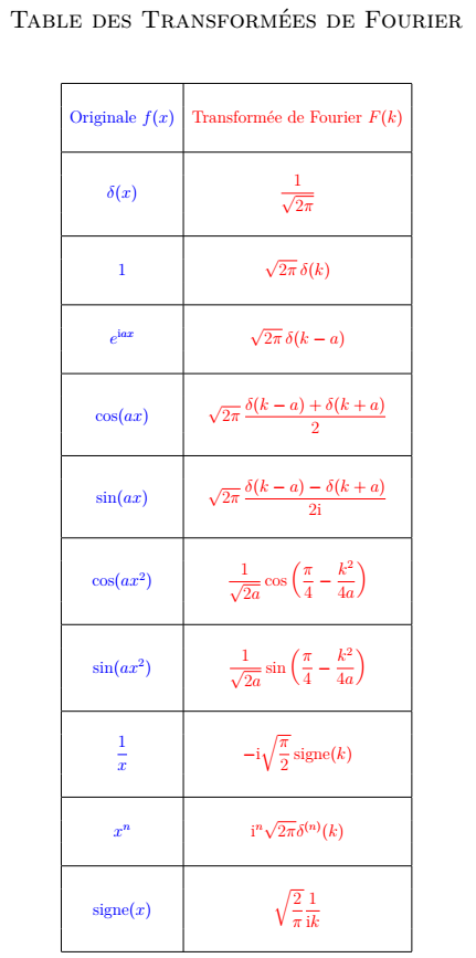
On donne la table suivante :
Question 1
On considère une poutre solide et homogène, mais déformable, linéaire, de longueur totale considérée comme infinie.
Physiquement, cela revient à pouvoir considérer que \textit{la longueur de la poutre est, au moins, cent fois plus importante que les autres distances caractéristique de la poutre}.
On désigne par la quantité réelle y(x ; t)y(x\,;\,t) la déformation transversale de la poutre à l'instant tt et à l'abscisse xx.
De fait la vitesse transversale vt=∂y∂tv_t = \dfrac{\partial y}{\partial t}. A l'instant initial t=0t=0, elle est donnée par l'expression :
vt(x ; t=0)=∂y∂t(x ; t=0)=ad2gdx2(x)    (a∈R+⋆)v_t(x \,;\, t=0) = \dfrac{\partial y}{\partial t}(x \,;\, t=0) = a \dfrac{\mathrm{d}^2 g}{\mathrm{d} x^2}(x) \,\,\,\, (a \in \mathbb{R}^{+\star})
où gg est une fonction numérique connue, continue et au moins deux fois dérivable sur l'intervalle [0 ; ℓ][0 \,;\, \ell].
A l'instant initial t=0t=0, la forme de la poutre est donnée par la relation suivante :
y(x ; t=0)=f(x)y(x\,;\,t=0) = f(x)
Puisque les vibrations sont libres (aucune force n'opère sur la poutre) on a l'équation du mouvement suivante :
∂4y∂x4(x ; t)+1a2∂2y∂t2(x ; t)=0    (a∈R+⋆)\dfrac{\partial^4 y}{\partial x^4}(x\,;\,t) + \dfrac{1}{a^2} \dfrac{\partial^2 y}{\partial t^2}(x\,;\,t) = 0 \,\,\,\, (a \in \mathbb{R}^{+\star})
On note par i\mathrm{i} le nombre imaginaire pur qui vérifie i2=−1\mathrm{i}^2 = -1. Dans cette partie, on adoptera, pour une fonction numérique ww, la définition de la \textit{Transformée de Fourier} suivante :
W(k)=TF[w(x)]=12π∫−∞+∞w(x) e−ikx dxW(k) = TF[w(x)] = \dfrac{1}{\sqrt{2\pi}} \int_{-\infty}^{+\infty} w(x) \, e^{-\mathrm{i}kx} \, \mathrm{d}x
De fait :
w(x)=TF−1[W(k)]=12π∫−∞+∞W(k) eikx dkw(x) = TF^{-1}[W(k)] = \dfrac{1}{\sqrt{2\pi}} \int_{-\infty}^{+\infty} W(k) \, e^{\mathrm{i}kx} \, \mathrm{d}k
C'est pourquoi on adoptera l'écriture suivante :
Y(k ; t)=TF[y(x ; t)]=12π∫−∞+∞y(x ; t) e−ikx dxY(k\,;\,t) = TF[y(x\,;\,t)] = \dfrac{1}{\sqrt{2\pi}} \int_{-\infty}^{+\infty} y(x\,;\,t) \, e^{-\mathrm{i}kx} \, \mathrm{d}x
On admettra que l'amplitude transversale de vibration yy satisfait à la condition physique suivante :
∀t∈R+,  lim⁡x⟶−∞y(x ; t)=lim⁡x⟶+∞y(x ; t)=0\forall t \in \mathbb{R}^+, \,\, \lim_{x \longrightarrow - \infty} y(x\,;\,t) = \lim_{x \longrightarrow + \infty} y(x\,;\,t) = 0
On notera par F(k)=TF[f(x)]=TF[y(x ; t=0)]F(k) = TF[f(x)] = TF[y(x\,;\,t=0)] et par G(k)=TF[g(x)]G(k) = TF[g(x)].

Déterminer l'expression de TF[∂y∂x(x ; t)]TF\left[\dfrac{\partial y}{\partial x}(x\,;\,t)\right] en fonction de Y(k ; t)Y(k\,;\,t).

Correction
On cherche :
TF[∂y∂x(x ; t)]=12π∫−∞+∞∂y∂x(x ; t) e−ikx dxTF\left[\dfrac{\partial y}{\partial x}(x\,;\,t)\right] = \dfrac{1}{\sqrt{2\pi}} \int_{-\infty}^{+\infty} \dfrac{\partial y}{\partial x}(x\,;\,t) \, e^{-\mathrm{i}kx} \, \mathrm{d}x
On constate immédiatement que l'expression ∂y∂x(x ; t)\dfrac{\partial y}{\partial x}(x\,;\,t) est une dérivée partielle selon la même variable que celle de l'intégration. Dans ce cas, le cours nous permet d'écrire que :
TF[∂y∂x(x ; t)]=ik 12π∫−∞+∞y(x ; t) e−ikx dxTF\left[\dfrac{\partial y}{\partial x}(x\,;\,t)\right] = \mathrm{i}k \, \dfrac{1}{\sqrt{2\pi}} \int_{-\infty}^{+\infty} y(x\,;\,t) \, e^{-\mathrm{i}kx} \, \mathrm{d}x
Ce qui nous donne :
TF[∂y∂x(x ; t)]=ik Y(k ; t)TF\left[\dfrac{\partial y}{\partial x}(x\,;\,t)\right] = \mathrm{i}k \, Y(k\,;\,t)
Question 2

En déduire l'expression de TF[∂4y∂x4(x ; t)]TF\left[\dfrac{\partial^4 y}{\partial x^4}(x\,;\,t)\right] en fonction de Y(k ; t)Y(k\,;\,t).

Correction
On cherche :
TF[∂4y∂x4(x ; t)]=12π∫−∞+∞∂4y∂x4(x ; t) e−ikx dxTF\left[\dfrac{\partial^4 y}{\partial x^4}(x\,;\,t)\right] = \dfrac{1}{\sqrt{2\pi}} \int_{-\infty}^{+\infty} \dfrac{\partial^4 y}{\partial x^4}(x\,;\,t) \, e^{-\mathrm{i}kx} \, \mathrm{d}x
On constate immédiatement que l'expression ∂4y∂x4(x ; t)\dfrac{\partial^4 y}{\partial x^4}(x\,;\,t) est une dérivée partielle selon la même variable que celle de l'intégration. Dans ce cas, le cours nous permet d'écrire que :
TF[∂4y∂x4(x ; t)]=(ik)4 12π∫−∞+∞y(x ; t) e−ikx dxTF\left[\dfrac{\partial^4 y}{\partial x^4}(x\,;\,t)\right] = (\mathrm{i}k)^4 \, \dfrac{1}{\sqrt{2\pi}} \int_{-\infty}^{+\infty} y(x\,;\,t) \, e^{-\mathrm{i}kx} \, \mathrm{d}x
Ce qui nous donne :
TF[∂4y∂x4(x ; t)]=(ik)4 Y(k ; t)TF\left[\dfrac{\partial^4 y}{\partial x^4}(x\,;\,t)\right] = (\mathrm{i}k)^4 \, Y(k\,;\,t)
D'où :
TF[∂4y∂x4(x ; t)]=i4k4 Y(k ; t)TF\left[\dfrac{\partial^4 y}{\partial x^4}(x\,;\,t)\right] = \mathrm{i}^4 k^4 \, Y(k\,;\,t)
Que nous allons écrire comme :
TF[∂4y∂x4(x ; t)]=(i2)2k4 Y(k ; t)TF\left[\dfrac{\partial^4 y}{\partial x^4}(x\,;\,t)\right] = \left(\mathrm{i}^2 \right)^2 k^4 \, Y(k\,;\,t)
Ainsi :
TF[∂4y∂x4(x ; t)]=(−1)2k4 Y(k ; t)TF\left[\dfrac{\partial^4 y}{\partial x^4}(x\,;\,t)\right] = \left(-1 \right)^2 k^4 \, Y(k\,;\,t)
Finalement :
TF[∂4y∂x4(x ; t)]=k4 Y(k ; t)TF\left[\dfrac{\partial^4 y}{\partial x^4}(x\,;\,t)\right] = k^4 \, Y(k\,;\,t)
Question 3

Déterminer l'expression de TF[∂y∂t(x ; t)]TF\left[\dfrac{\partial y}{\partial t}(x\,;\,t)\right].

Correction
On cherche :
TF[∂y∂t(x ; t)]=12π∫−∞+∞∂y∂t(x ; t) e−ikx dxTF\left[\dfrac{\partial y}{\partial t}(x\,;\,t)\right] = \dfrac{1}{\sqrt{2\pi}} \int_{-\infty}^{+\infty} \dfrac{\partial y}{\partial t}(x\,;\,t) \, e^{-\mathrm{i}kx} \, \mathrm{d}x
On constate immédiatement que l'expression ∂y∂t(x ; t)\dfrac{\partial y}{\partial t}(x\,;\,t) est une dérivée partielle selon la variable temporelle tt. Mais, l'intégration s'effectue selon la variable spatiale xx. De fait, la permutation des opérateur de dérivation partielle et d'intégration est possible. Dans ce cas, on obtient :
TF[∂y∂t(x ; t)]=12π∂∂t∫−∞+∞y(x ; t) e−ikx dxTF\left[\dfrac{\partial y}{\partial t}(x\,;\,t)\right] = \dfrac{1}{\sqrt{2\pi}} \dfrac{\partial }{\partial t}\int_{-\infty}^{+\infty} y(x\,;\,t) \, e^{-\mathrm{i}kx} \, \mathrm{d}x
Soit :
TF[∂y∂t(x ; t)]=∂∂t12π∫−∞+∞y(x ; t) e−ikx dxTF\left[\dfrac{\partial y}{\partial t}(x\,;\,t)\right] = \dfrac{\partial }{\partial t} \dfrac{1}{\sqrt{2\pi}} \int_{-\infty}^{+\infty} y(x\,;\,t) \, e^{-\mathrm{i}kx} \, \mathrm{d}x
Soit encore :
TF[∂y∂t(x ; t)]=∂∂tY(k ; t)TF\left[\dfrac{\partial y}{\partial t}(x\,;\,t)\right] = \dfrac{\partial }{\partial t} Y(k\,;\,t)
Finalement :
TF[∂y∂t(x ; t)]=∂Y∂t(k ; t)TF\left[\dfrac{\partial y}{\partial t}(x\,;\,t)\right] = \dfrac{\partial Y}{\partial t} (k\,;\,t)
Question 4

Déterminer l'expression de TF[∂2y∂t2(x ; t)]TF\left[\dfrac{\partial^2 y}{\partial t^2}(x\,;\,t)\right].

Correction
On cherche :
TF[∂2y∂t2(x ; t)]=12π∫−∞+∞∂y∂t(x ; t) e−ikx dxTF\left[\dfrac{\partial^2 y}{\partial t^2}(x\,;\,t)\right] = \dfrac{1}{\sqrt{2\pi}} \int_{-\infty}^{+\infty} \dfrac{\partial y}{\partial t}(x\,;\,t) \, e^{-\mathrm{i}kx} \, \mathrm{d}x
De la même manière qu'à la question précédente, on constate immédiatement que l'expression ∂2y∂t2(x ; t)\dfrac{\partial^2 y}{\partial t^2}(x\,;\,t) est une dérivée partielle seconde selon la variable temporelle tt. Mais, l'intégration s'effectue selon la variable spatiale xx. De fait, la permutation des opérateur de dérivation partielle et d'intégration est possible. Dans ce cas, on obtient :
TF[∂2y∂t2(x ; t)]=12π∂2∂t2∫−∞+∞y(x ; t) e−ikx dxTF\left[\dfrac{\partial^2 y}{\partial t^2}(x\,;\,t)\right] = \dfrac{1}{\sqrt{2\pi}} \dfrac{\partial^2 }{\partial t^2}\int_{-\infty}^{+\infty} y(x\,;\,t) \, e^{-\mathrm{i}kx} \, \mathrm{d}x
Soit :
TF[∂y2∂t2(x ; t)]=∂2∂t212π∫−∞+∞y(x ; t) e−ikx dxTF\left[\dfrac{\partial y^2}{\partial t^2}(x\,;\,t)\right] = \dfrac{\partial^2 }{\partial t^2} \dfrac{1}{\sqrt{2\pi}} \int_{-\infty}^{+\infty} y(x\,;\,t) \, e^{-\mathrm{i}kx} \, \mathrm{d}x
Soit encore :
TF[∂2y∂t2(x ; t)]=∂2∂t2Y(k ; t)TF\left[\dfrac{\partial^2 y}{\partial t^2}(x\,;\,t)\right] = \dfrac{\partial^2 }{\partial t^2} Y(k\,;\,t)
Finalement :
TF[∂2y∂t2(x ; t)]=∂2Y∂t2(k ; t)TF\left[\dfrac{\partial^2 y}{\partial t^2}(x\,;\,t)\right] = \dfrac{\partial^2 Y}{\partial t^2} (k\,;\,t)
Question 5

Déterminer les dimensions physiques de la constante réelle aa.

Correction
Le sujet nous donne l'Equation aux Dérivées Partielles (E.D.P.) suivante :
∂4y∂x4(x ; t)+1a2∂2y∂t2(x ; t)=0    (a∈R+⋆)\dfrac{\partial^4 y}{\partial x^4}(x\,;\,t) + \dfrac{1}{a^2} \dfrac{\partial^2 y}{\partial t^2}(x\,;\,t) = 0 \,\,\,\, (a \in \mathbb{R}^{+\star})
Cette E.D.P. est la traduction mathématique d'une loi physique. La Physique devant être homogène par ses dimensions, nous pouvons donc écrire que :
dim⁡(∂4y∂x4(x ; t))=dim⁡(1a2∂2y∂t2(x ; t))\dim \left( \dfrac{\partial^4 y}{\partial x^4}(x\,;\,t) \right) = \dim \left( \dfrac{1}{a^2} \dfrac{\partial^2 y}{\partial t^2}(x\,;\,t) \right)
Soit :
dim⁡(∂4y∂x4(x ; t))=dim⁡(1a2)×dim⁡(∂2y∂t2(x ; t))\dim \left( \dfrac{\partial^4 y}{\partial x^4}(x\,;\,t) \right) = \dim \left( \dfrac{1}{a^2} \right) \times \dim \left( \dfrac{\partial^2 y}{\partial t^2}(x\,;\,t) \right)
Soit encore :
dim⁡(∂4y∂x4(x ; t))=1(dim⁡(a))2×dim⁡(∂2y∂t2(x ; t))\dim \left( \dfrac{\partial^4 y}{\partial x^4}(x\,;\,t) \right) = \dfrac{1}{\left( \dim \left( a \right)\right)^2} \times \dim \left( \dfrac{\partial^2 y}{\partial t^2}(x\,;\,t) \right)
D'où :
dim⁡(y)(dim⁡(x))4=1(dim⁡(a))2×dim⁡(y)(dim⁡(t))2\dfrac{\dim \left( y \right)}{\left(\dim \left( x\right)\right)^4} = \dfrac{1}{\left( \dim \left( a \right)\right)^2} \times \dfrac{\dim \left( y \right)}{\left(\dim \left( t \right)\right)^2}
Or, dim⁡(y)=L=dim⁡(x)\dim \left( y \right) = L = \dim \left( x \right) et dim⁡(t)=T\dim \left( t \right) = T. Ainsi, on obtient :
LL4=1(dim⁡(a))2×LT2\dfrac{L}{L^4} = \dfrac{1}{\left( \dim \left( a \right)\right)^2} \times \dfrac{L}{T^2}
En simplifiant :
1L3=1(dim⁡(a))2×LT2\dfrac{1}{L^3} = \dfrac{1}{\left( \dim \left( a \right)\right)^2} \times \dfrac{L}{T^2}
Donc :
(dim⁡(a))2=L.L3T2\left( \dim \left( a \right)\right)^2 = \dfrac{L.L^3}{T^2}
Ce qui nous permet d'écrire que :
(dim⁡(a))2=L4T2\left( \dim \left( a \right)\right)^2 = \dfrac{L^4}{T^2}
Mais également :
(dim⁡(a))2=(L2T)2\left( \dim \left( a \right)\right)^2 = \left( \dfrac{L^2}{T} \right)^2
On en déduit alors que :
dim⁡(a)=L2T\dim \left( a \right) = \dfrac{L^2}{T}
Finalement :
dim⁡(a)=L2.T−1\dim \left( a \right) = L^2.T^{-1}
Ainsi la constante aa possède la dimension d'une surface par unité de temps ; ce qui est identique à une diffusivité.
Question 6

A l'aide de la \textit{Transformée de Fourier}, démontrer que :
y(x ; t)=12π∫−∞+∞F(k) cos⁡(ak2t) eikx dk−12π∫−∞+∞G(k) sin⁡(ak2t) eikx dky(x \,;\,t) = \dfrac{1}{\sqrt{2\pi}} \int_{-\infty}^{+\infty} F(k) \, \cos(ak^2t) \, e^{\mathrm{i}kx} \, \mathrm{d}k - \dfrac{1}{\sqrt{2\pi}} \int_{-\infty}^{+\infty} G(k) \, \sin(ak^2t) \, e^{\mathrm{i}kx} \, \mathrm{d}k

Correction
Prenons la transformée de Fourier de l'E.D.P. proposée par le sujet. On a :
TF[∂4y∂x4(x ; t)+1a2∂2y∂t2(x ; t)]=TF[0]TF\left[ \dfrac{\partial^4 y}{\partial x^4}(x\,;\,t) + \dfrac{1}{a^2} \dfrac{\partial^2 y}{\partial t^2}(x\,;\,t) \right] = TF\left[ 0 \right]
Par linéarité de la transformation de Fourier, on a alors :
TF[∂4y∂x4(x ; t)]+TF[1a2∂2y∂t2(x ; t)]=TF[0]TF\left[ \dfrac{\partial^4 y}{\partial x^4}(x\,;\,t) \right] + TF\left[ \dfrac{1}{a^2} \dfrac{\partial^2 y}{\partial t^2}(x\,;\,t) \right] = TF\left[ 0 \right]
Comme aa est une constante réelle, on a alors :
TF[∂4y∂x4(x ; t)]+1a2 TF[∂2y∂t2(x ; t)]=TF[0]TF\left[ \dfrac{\partial^4 y}{\partial x^4}(x\,;\,t) \right] + \dfrac{1}{a^2} \, TF\left[ \dfrac{\partial^2 y}{\partial t^2}(x\,;\,t) \right] = TF\left[ 0 \right]
De plus, on sait que TF[0]=0TF\left[ 0 \right] = 0. Donc :
TF[∂4y∂x4(x ; t)]+1a2 TF[∂2y∂t2(x ; t)]=0TF\left[ \dfrac{\partial^4 y}{\partial x^4}(x\,;\,t) \right] + \dfrac{1}{a^2} \, TF\left[ \dfrac{\partial^2 y}{\partial t^2}(x\,;\,t) \right] = 0
En faisant usage, maintenant, des résultats précédents, on peut donc écrire que :
k4 Y(k ; t)+1a2 ∂2Y∂t2(k ; t)=0k^4 \, Y(k\,;\,t) + \dfrac{1}{a^2} \, \dfrac{\partial^2 Y}{\partial t^2} (k\,;\,t) = 0
Ce qui nous donne aussi :
a2k4 Y(k ; t)+∂2Y∂t2(k ; t)=0a^2 k^4 \, Y(k\,;\,t) + \dfrac{\partial^2 Y}{\partial t^2} (k\,;\,t) = 0
Que nous allons écrire sous la forme :
∂2Y∂t2(k ; t)+(ak2)2 Y(k ; t)=0\dfrac{\partial^2 Y}{\partial t^2} (k\,;\,t) + \left( a k^2 \right)^2 \, Y(k\,;\,t) = 0
Cette équation est celle d'un oscillateur harmonique temporel de pulsation ω=ak2\omega = ak^2. Les solutions de cette équations sont classiques et bien connues. Afin de tenir compte de la dépendance en k{\color{red}{k}}, ces solutions Y(k ; t)Y({\color{red}{k}}\,;\,t) sont de la forme :
Y(k ; t)=A(k) cos⁡(ω t)+B(k) sin⁡(ω t)Y({\color{red}{k}}\,;\,t) = A({\color{red}{k}}) \, \cos(\omega \, t) + B({\color{red}{k}}) \, \sin(\omega \, t)
Soit :
Y(k ; t)=A(k) cos⁡(ak2 t)+B(k) sin⁡(ak2 t)Y({\color{red}{k}}\,;\,t) = A({\color{red}{k}}) \, \cos(ak^2 \, t) + B({\color{red}{k}}) \, \sin(ak^2 \, t)
Faisons maintenant usage des deux conditions limites données par le sujet.
A l'instant initial t=0t=0, la forme de la poutre est donnée par la relation suivante :
y(x ; t=0)=f(x)y(x\,;\,t=0) = f(x)
Ce qui implique, en prenant la transformée de Fourier de cette relation, que :
TF[y(x ; t=0)]=TF[f(x)]    ⟺    Y(k ; t=0)=F(k)TF \left[ y(x\,;\,t=0) \right] = TF \left[ f(x) \right] \,\,\,\, \Longleftrightarrow \,\,\,\, Y(k\,;\,t=0) = F(k)
Or, on constate que :
Y(k ; t=0)=A(k) cos⁡(ak2 0)+B(k) sin⁡(ak2 0)Y({\color{red}{k}}\,;\,t=0) = A({\color{red}{k}}) \, \cos(ak^2 \, 0) + B({\color{red}{k}}) \, \sin(ak^2 \, 0)
Soit :
Y(k ; 0)=A(k) cos⁡(0)+B(k) sin⁡(0)Y({\color{red}{k}}\,;\,0) = A({\color{red}{k}}) \, \cos(0) + B({\color{red}{k}}) \, \sin(0)
Soit encore :
Y(k ; 0)=A(k) 1+B(k) 0Y({\color{red}{k}}\,;\,0) = A({\color{red}{k}}) \, 1 + B({\color{red}{k}}) \, 0
Donc :
Y(k ; 0)=A(k)Y({\color{red}{k}}\,;\,0) = A({\color{red}{k}})
Ce qui nous permet d'écrire que :
F(k)=A(k)F(k) = A({\color{red}{k}})
Donc, à ce stade, on obtient :
Y(k ; t)=F(k) cos⁡(ak2 t)+B(k) sin⁡(ak2 t)Y({\color{red}{k}}\,;\,t) = F({\color{red}{k}}) \, \cos(ak^2 \, t) + B({\color{red}{k}}) \, \sin(ak^2 \, t)
De plus, à l'instant initial t=0t=0, la vitesse transversale est donnée par l'expression :
vt(x ; t=0)=∂y∂t(x ; t=0)=ad2gdx2(x)v_t(x \,;\, t=0) = \dfrac{\partial y}{\partial t}(x \,;\, t=0) = a \dfrac{\mathrm{d}^2 g}{\mathrm{d} x^2}(x)
Donc, en prenant la transformée de Fourier de cette relation, on obtient :
TF[∂y∂t(x ; t=0)]=TF[ad2gdx2(x)]TF \left[ \dfrac{\partial y}{\partial t}(x \,;\, t=0) \right] = TF \left[ a \dfrac{\mathrm{d}^2 g}{\mathrm{d} x^2}(x) \right]
Soit :
TF[∂y∂t(x ; t=0)]=a TF[d2gdx2(x)]TF \left[ \dfrac{\partial y}{\partial t}(x \,;\, t=0) \right] = a \, TF \left[ \dfrac{\mathrm{d}^2 g}{\mathrm{d} x^2}(x) \right]
Soit :
∂∂tTF[y(x ; t=0)]=a (ik)2 TF[g(x)]\dfrac{\partial }{\partial t} TF \left[ y(x \,;\, t=0) \right] = a \, ( \mathrm{i} k)^2 \, TF \left[ g(x) \right]
Avec (ik)2=i2k2=−1×k=−k( \mathrm{i} k)^2 = \mathrm{i}^2 k^2 = -1 \times k = - k, on obtient :
∂∂tY(k ; 0)=−a k2 G(k)\dfrac{\partial }{\partial t} Y({\color{red}{k}}\,;\,0) = - a \, k^2 \, G(k)
D'où :
∂Y∂t(k ; 0)=−a k2 G(k)\dfrac{\partial Y}{\partial t} ({\color{red}{k}}\,;\,0) = - a \, k^2 \, G(k)
Ce qui nous donne :
∂Y∂t(F(k) cos⁡(ak2 t)+B(k) sin⁡(ak2 t))t=0=−a k2 G(k)\dfrac{\partial Y}{\partial t} \left( F({\color{red}{k}}) \, \cos(ak^2 \, t) + B({\color{red}{k}}) \, \sin(ak^2 \, t) \right)_{t=0} = - a \, k^2 \, G(k)
Par linéarité de la dérivation partielle temporelle, on a alors :
F(k) ∂Y∂t(cos⁡(ak2 t))t=0+B(k) ∂Y∂t(sin⁡(ak2 t))t=0=<br/>−a k2 G(k)F({\color{red}{k}}) \, \dfrac{\partial Y}{\partial t} \left( \cos(ak^2 \, t) \right)_{t=0} + B({\color{red}{k}}) \, \dfrac{\partial Y}{\partial t} \left( \sin(ak^2 \, t) \right)_{t=0} = <br />- a \, k^2 \, G(k)
On obtient :
F(k) (−ak2)sin⁡(ak2 0)+B(k) ak2cos⁡(ak2 0)=−a k2 G(k)F({\color{red}{k}}) \, \left( - ak^2 \right) \sin(ak^2 \, 0) + B({\color{red}{k}}) \, ak^2 \cos(ak^2 \, 0) = - a \, k^2 \, G(k)
D'où :
−ak2 F(k) sin⁡(ak2 0)+ak2 B(k) cos⁡(ak2 0)=−a k2 G(k)- ak^2 \, F({\color{red}{k}}) \, \sin(ak^2 \, 0) + ak^2 \, B({\color{red}{k}}) \, \cos(ak^2 \, 0) = - a \, k^2 \, G(k)
Par simplification par le terme non nul toujours nul −ak2- ak^2, on arrive à :
F(k) sin⁡(ak2 0)−B(k) cos⁡(ak2 0)=<br/>G(k)F({\color{red}{k}}) \, \sin(ak^2 \, 0) - B({\color{red}{k}}) \, \cos(ak^2 \, 0) = <br />G(k)
Soit :
F(k) sin⁡(0)−B(k) cos⁡(0)=G(k)F({\color{red}{k}}) \, \sin(0) - B({\color{red}{k}}) \, \cos(0) = G(k)
Soit encore :
F(k) 0−B(k) 1=G(k)F({\color{red}{k}}) \, 0 - B({\color{red}{k}}) \, 1 = G(k)
Donc :
−B(k)=G(k)- B({\color{red}{k}}) = G(k)
Et :
B(k)=−G(k)B({\color{red}{k}}) = - G(k)
On arrive donc au résultat suivant :
Y(k ; t)=F(k) cos⁡(ak2 t)−G(k) sin⁡(ak2 t)Y({\color{red}{k}}\,;\,t) = F({\color{red}{k}}) \, \cos(ak^2 \, t) - G({\color{red}{k}}) \, \sin(ak^2 \, t)
En prenant la transformée de Fourier inverse de cette dernière relation, nous obtenons :
TF−1[Y(k ; t)]=TF−1[F(k) cos⁡(ak2 t)−G(k) sin⁡(ak2 t)]TF^{-1} \left[ Y({\color{red}{k}}\,;\,t) \right] = TF^{-1} \left[ F({\color{red}{k}}) \, \cos(ak^2 \, t) - G({\color{red}{k}}) \, \sin(ak^2 \, t) \right]
Puis, par linéarité, nous obtenons :
TF−1[Y(k ; t)]=TF−1[F(k) cos⁡(ak2 t)]−TF−1[G(k) sin⁡(ak2 t)]TF^{-1} \left[ Y({\color{red}{k}}\,;\,t) \right] = TF^{-1} \left[ F({\color{red}{k}}) \, \cos(ak^2 \, t) \right] - TF^{-1} \left[ G({\color{red}{k}}) \, \sin(ak^2 \, t) \right]
Soit :
y(x ; t)=TF−1[F(k) cos⁡(ak2 t)]−TF−1[G(k) sin⁡(ak2 t)]y(x \,;\,t) = TF^{-1} \left[ F({\color{red}{k}}) \, \cos(ak^2 \, t) \right] - TF^{-1} \left[ G({\color{red}{k}}) \, \sin(ak^2 \, t) \right]
Finalement, on obtient bien l'expression proposée par le sujet, à savoir :
y(x ; t)=12π∫−∞+∞F(k) cos⁡(ak2t) eikx dk−12π∫−∞+∞G(k) sin⁡(ak2t) eikx dky(x \,;\,t) = \dfrac{1}{\sqrt{2\pi}} \int_{-\infty}^{+\infty} F(k) \, \cos(ak^2t) \, e^{\mathrm{i}kx} \, \mathrm{d}k - \dfrac{1}{\sqrt{2\pi}} \int_{-\infty}^{+\infty} G(k) \, \sin(ak^2t) \, e^{\mathrm{i}kx} \, \mathrm{d}k
Question 7

Démontrer que :
y(x ; t)=12πat(∫−∞+∞f(x−h) cos⁡(h24a−π4) dh+∫−∞+∞g(x−h) sin⁡(h24a−π4) dh)y(x \,;\,t) = \dfrac{1}{2\sqrt{\pi a t}} \left( \int_{-\infty}^{+\infty} f(x - h) \, \cos\left( \dfrac{h^2}{4a} - \dfrac{\pi}{4} \right) \, \mathrm{d}h + \int_{-\infty}^{+\infty} g(x - h) \, \sin\left( \dfrac{h^2}{4a} - \dfrac{\pi}{4} \right) \, \mathrm{d}h \right)
La lettre hh représente, dans la formule précédente, est une variable d'intégration muette. De fait, vous pouvez lui donner une autre dénomination (autre qu'une celle déjà utilisée auparavant).

Correction
Or, la table de correspondance qui est donnée avec le sujet de cet exercice, nous apprends que :
{TF[cos⁡(βx2)]=12βcos⁡(π4−k24β)TF[sin⁡(βx2)]=12βsin⁡(π4−k24β)     (β∈R)\left\lbrace \begin{array}{rcl} TF\left[ {\color{blue}{\cos(\beta x^2)}} \right] & = & {\color{red}{\dfrac{1}{\sqrt{2\beta}}\cos\left( \dfrac{\pi}{4} - \dfrac{k^2}{4\beta} \right)}} \\ & & \\ TF\left[ {\color{blue}{\sin(\beta x^2)}} \right] & = & {\color{red}{\dfrac{1}{\sqrt{2\beta}}\sin\left( \dfrac{\pi}{4} - \dfrac{k^2}{4\beta} \right)}} \\ \end{array} \right. \,\,\,\,\, (\beta \in \mathbb{R})
Donc, par réciprocité, on en déduit que :
{TF−1[cos⁡(βk2)]=12βcos⁡(π4−x24β)TF−1[sin⁡(βk2)]=12βsin⁡(π4−x24β)     (β∈R)\left\lbrace\begin{array}{rcl} TF^{-1}\left[ {\color{blue}{\cos(\beta k^2)}} \right] & = & {\color{red}{\dfrac{1}{\sqrt{2\beta}}\cos\left( \dfrac{\pi}{4} - \dfrac{x^2}{4\beta} \right)}} \\ & & \\ TF^{-1}\left[ {\color{blue}{\sin(\beta k^2)}} \right] & = & {\color{red}{\dfrac{1}{\sqrt{2\beta}}\sin\left( \dfrac{\pi}{4} - \dfrac{x^2}{4\beta} \right)}} \\ \end{array} \right. \,\,\,\,\, (\beta \in \mathbb{R})
En tenant compte de la parité de cosinus et de l'imparité de sinus on obtient :
{TF−1[cos⁡(βk2)]=12βcos⁡(x24β−π4)TF−1[sin⁡(βk2)]=−12βsin⁡(x24β−π4)     (β∈R)\left\lbrace \begin{array}{rcl} TF^{-1}\left[ {\color{blue}{\cos(\beta k^2)}} \right] & = & {\color{red}{\dfrac{1}{\sqrt{2\beta}}\cos\left( \dfrac{x^2}{4\beta} - \dfrac{\pi}{4} \right)}} \\ & & \\ TF^{-1}\left[ {\color{blue}{\sin(\beta k^2)}} \right] & = & {\color{red}{- \dfrac{1}{\sqrt{2\beta}}\sin\left( \dfrac{x^2}{4\beta} - \dfrac{\pi}{4} \right)}} \\ \end{array} \right. \,\,\,\,\, (\beta \in \mathbb{R})
Et de fait :
{TF−1[cos⁡(βk2)]=12βcos⁡(x24β−π4)TF−1[−sin⁡(βk2)]=12βsin⁡(x24β−π4)     (β∈R)\left\lbrace \begin{array}{rcl} TF^{-1}\left[ {\color{blue}{\cos(\beta k^2)}} \right] & = & {\color{red}{\dfrac{1}{\sqrt{2\beta}}\cos\left( \dfrac{x^2}{4\beta} - \dfrac{\pi}{4} \right)}} \\ & & \\ TF^{-1}\left[ {\color{blue}{- \sin(\beta k^2)}} \right] & = & {\color{red}{\dfrac{1}{\sqrt{2\beta}}\sin\left( \dfrac{x^2}{4\beta} - \dfrac{\pi}{4} \right)}} \\ \end{array} \right. \,\,\,\,\, (\beta \in \mathbb{R})
Posons maintenant β=at\beta = at. On obtient donc les deux relations suivantes :
{TF−1[cos⁡(atk2)]=12atcos⁡(x24at−π4)TF−1[−sin⁡(atk2)]=12atsin⁡(x24at−π4)\left\lbrace \begin{array}{rcl} TF^{-1}\left[ {\color{blue}{\cos(at k^2)}} \right] & = & {\color{red}{\dfrac{1}{\sqrt{2at}}\cos\left( \dfrac{x^2}{4at} - \dfrac{\pi}{4} \right)}} \\ & & \\ TF^{-1}\left[ {\color{blue}{- \sin(at k^2)}} \right] & = & {\color{red}{\dfrac{1}{\sqrt{2at}}\sin\left( \dfrac{x^2}{4at} - \dfrac{\pi}{4} \right)}} \\ \end{array} \right.
En prenant maintenant la transformée de Fourier de ces deux expressions, membre à membre, on obtient :
{cos⁡(atk2)=TF[12atcos⁡(x24at−π4)]−sin⁡(atk2)=TF[12atsin⁡(x24at−π4)]\left\lbrace \begin{array}{rcl} {\color{blue}{\cos(at k^2)}} & = & TF \left[ {\color{red}{\dfrac{1}{\sqrt{2at}}\cos\left( \dfrac{x^2}{4at} - \dfrac{\pi}{4} \right)}} \right] \\ & & \\ {\color{blue}{- \sin(at k^2)}} & = & TF \left[ {\color{red}{\dfrac{1}{\sqrt{2at}} \sin\left( \dfrac{x^2}{4at} - \dfrac{\pi}{4} \right)}} \right] \\ \end{array} \right.
Ainsi, le résultat de la question précédente prend la forme suivante :
y(x ; t)=12π∫−∞+∞TF[f(x)]×TF[12atcos⁡(x24at−π4)] eikx dk+12π∫−∞+∞TF[g(x)]×TF[12atsin⁡(x24at−π4)] eikx dk\begin{array}{rcl}y(x \,;\,t) & = & \dfrac{1}{\sqrt{2\pi}} \displaystyle{ \int_{- \infty}^{+\infty} } TF[f(x)] \times TF \left[ {\color{red}{\dfrac{1}{\sqrt{2at}}\cos\left( \dfrac{x^2}{4at} - \dfrac{\pi}{4} \right)}} \right] \, e^{\mathrm{i}kx} \, \mathrm{d}k \\ & & \\ & + & \dfrac{1}{\sqrt{2\pi}} \displaystyle{ \int_{-\infty}^{+\infty} } TF[g(x)] \times TF \left[ {\color{red}{\dfrac{1}{\sqrt{2at}}\sin\left( \dfrac{x^2}{4at} - \dfrac{\pi}{4} \right)}} \right] \, e^{\mathrm{i}kx} \, \mathrm{d}k \end{array}
Soit :
y(x ; t)=TF−1[TF[f(x)]×TF[12atcos⁡(x24at−π4)]]+TF−1[TF[g(x)]×TF[12atsin⁡(x24at−π4)]]\begin{array}{rcl} y(x \,;\,t) & = & TF^{-1}\left[ TF[f(x)] \times TF \left[ {\color{red}{\dfrac{1}{\sqrt{2at}}\cos\left( \dfrac{x^2}{4at} - \dfrac{\pi}{4} \right)}} \right] \right] \\ & & \\ & + & TF^{-1}\left[ TF[g(x)] \times TF \left[ {\color{red}{\dfrac{1}{\sqrt{2at}}\sin\left( \dfrac{x^2}{4at} - \dfrac{\pi}{4} \right)}} \right] \right] \end{array}
D'après le cours, on voit apparaitre un produit de convolution, de symbole ⋆\star, qui va permettre d'exprimer simplement la solution recherchée. On a alors :
y(x ; t)=TF−1[TF[12π f(x)⋆12atcos⁡(x24at−π4)]]+TF−1[TF[12π g(x)⋆12atsin⁡(x24at−π4)]]\begin{array}{rcl} y(x \,;\,t) & = & TF^{-1}\left[ TF \left[ \dfrac{1}{\sqrt{2\pi}} \, f(x) \star {\color{red}{\dfrac{1}{\sqrt{2at}}\cos\left( \dfrac{x^2}{4at} - \dfrac{\pi}{4} \right)}} \right] \right] \\ & & \\ & + & TF^{-1}\left[ TF \left[ \dfrac{1}{\sqrt{2\pi}} \, g(x) \star {\color{red}{\dfrac{1}{\sqrt{2at}}\sin\left( \dfrac{x^2}{4at} - \dfrac{\pi}{4} \right)}} \right] \right] \end{array}
Or les opérations successives TF−1TF^{-1} et TFTF s'annulent. Ce qui nous donne donc :
y(x ; t)=12π f(x)⋆12atcos⁡(x24at−π4)+12π g(x)⋆12atsin⁡(x24at−π4)\begin{array}{rcl} y(x \,;\,t) & = & \dfrac{1}{\sqrt{2\pi}} \, f(x) \star {\color{red}{\dfrac{1}{\sqrt{2at}}\cos\left( \dfrac{x^2}{4at} - \dfrac{\pi}{4} \right)}} \\ & & \\ & + & \dfrac{1}{\sqrt{2\pi}} \, g(x) \star {\color{red}{\dfrac{1}{\sqrt{2at}}\sin\left( \dfrac{x^2}{4at} - \dfrac{\pi}{4} \right)}} \end{array}
Soit :
y(x ; t)=12π12at f(x)⋆cos⁡(x24at−π4)+12π12at g(x)⋆sin⁡(x24at−π4)\begin{array}{rcl} y(x \,;\,t) & = & \dfrac{1}{\sqrt{2\pi}} {\color{red}{\dfrac{1}{\sqrt{2at}}}} \, f(x) \star {\color{red}{\cos\left( \dfrac{x^2}{4at} - \dfrac{\pi}{4} \right)}} \\ & & \\ & + & \dfrac{1}{\sqrt{2\pi}} {\color{red}{\dfrac{1}{\sqrt{2at}}}} \, g(x) \star {\color{red}{\sin\left( \dfrac{x^2}{4at} - \dfrac{\pi}{4} \right)}} \end{array}
Soit encore :
y(x ; t)=12πat f(x)⋆cos⁡(x24at−π4)+12πat g(x)⋆sin⁡(x24at−π4)\begin{array}{rcl} y(x \,;\,t) & = & \dfrac{1}{2\sqrt{\pi at }} \, f(x) \star {\color{red}{\cos\left( \dfrac{x^2}{4at} - \dfrac{\pi}{4} \right)}} \\ & & \\ & + & \dfrac{1}{2\sqrt{\pi at }} \, g(x) \star {\color{red}{\sin\left( \dfrac{x^2}{4at} - \dfrac{\pi}{4} \right)}} \end{array}
Par factorisation du terme commun 12πat\dfrac{1}{2\sqrt{\pi at }}, on trouve que :
y(x ; t)=12πat(f(x)⋆cos⁡(x24at−π4)+g(x)⋆sin⁡(x24at−π4))y(x \,;\,t) = \dfrac{1}{2\sqrt{\pi at }} \left( f(x) \star {\color{red}{\cos\left( \dfrac{x^2}{4at} - \dfrac{\pi}{4} \right)}} + g(x) \star {\color{red}{\sin\left( \dfrac{x^2}{4at} - \dfrac{\pi}{4} \right)}} \right)
Finalement, en faisant usage de la définition intégrale du produit de convolution, on trouve bien la solution proposée par l'énoncé de cet exercice. En introduisant la lettre hh comme une variable d'intégration muette, on obtient l'expression recherchée, à savoir :
y(x ; t)=12πat(∫−∞+∞f(x−h) cos⁡(x24at−π4) dh+∫−∞+∞g(x−h) sin⁡(x24at−π4) dh)y(x \,;\,t) = \dfrac{1}{2\sqrt{\pi a t}} \left( \int_{-\infty}^{+\infty} f(x - h) \, {\color{red}{\cos\left( \dfrac{x^2}{4at} - \dfrac{\pi}{4} \right)}} \, \mathrm{d}h + \int_{-\infty}^{+\infty} g(x - h) \, {\color{red}{\sin\left( \dfrac{x^2}{4at} - \dfrac{\pi}{4} \right)}} \, \mathrm{d}h \right)
Question 8
Partie 2 - Poutre libre de longueur infinie de forme gaussienne{\color{RoyalBlue}{\textbf{Partie 2 - Poutre libre de longueur infinie de forme gaussienne}}}

On reprend la situation de la partie précédente.
On considère une poutre solide et homogène, mais déformable, linéaire, de longueur totale considérée comme infinie.
Physiquement, cela revient à pouvoir considérer que la longueur de la poutre est, au moins, cent fois plus importante que les autres distances caractéristique de la poutre.
Les conditions initiales vont être telles que la vitesse initiale transversale soit nulle sur toute la poutre. De fait cela impose que :
∀x∈R,  g(x)=0\forall x \in \mathbb{R}, \,\, g(x) = 0
Puis, la poutre va avoir initialement une forme gaussienne. Ceci va se traduire mathématiquement par la relation suivante :
∀x∈R,  f(x)=ε e−x24r2    avec (ε ; r)∈R+⋆2\forall x \in \mathbb{R}, \,\, f(x) = \varepsilon \, e^{- \frac{x^2}{4r^2}} \,\,\,\, \mathrm{avec} \, (\varepsilon \,;\,r) \in {\mathbb{R}^{+\star}}^2
Cette modélisation permet de décrire le comportement oscillant vertical d'un pont de très grande taille.

En vous aidant de la Partie 1{\color{RoyalBlue}{\textbf{Partie 1}}} précédente et des conditions initiales indiquées (et éventuellement des tables fournies avec cet énoncé), démontrer que l'on a le résultat suivant :
y(x ; t)=εr(r4+a2t2)14e−r2x24(r4+a2t2)cos⁡(atx24(r4+a2t2)−12arctan⁡(atr2))y(x \,;\,t) = \dfrac{\varepsilon r}{\left( r^4 + a^2t^2 \right)^{\frac{1}{4}} } e^{-\frac{r^2x^2}{4\left( r^4 + a^2t^2 \right) }} \cos \left( \dfrac{atx^2}{4\left( r^4 + a^2t^2 \right) } - \dfrac{1}{2} \arctan \left( \dfrac{at}{r^2} \right) \right)

Correction
Cette fois, les conditions initiales vont être telles que la vitesse initiale transversale est nulle sur toute la poutre. De fait cela implique que la fonction gg s'identifie à la fonction nulle. Ceci nous permet d'écrire que :
g=0x    ⟹    G=0kg = 0_x \,\,\,\, \Longrightarrow \,\,\,\, G=0_k
Selon la Partie 1{\color{RoyalBlue}{\textbf{Partie 1}}} précédente, on en déduit que :
y(x ; t)=12π∫−∞+∞F(k) cos⁡(ak2t) eikx dk−12π∫−∞+∞0 sin⁡(ak2t) eikx dky(x \,;\,t) = \dfrac{1}{\sqrt{2\pi}} \int_{-\infty}^{+\infty} F(k) \, \cos(ak^2t) \, e^{\mathrm{i}kx} \, \mathrm{d}k - \dfrac{1}{\sqrt{2\pi}} \int_{-\infty}^{+\infty} 0 \, \sin(ak^2t) \, e^{\mathrm{i}kx} \, \mathrm{d}k
Ce qui nous donne :
y(x ; t)=12π∫−∞+∞F(k) cos⁡(ak2t) eikx dky(x \,;\,t) = \dfrac{1}{\sqrt{2\pi}} \int_{-\infty}^{+\infty} F(k) \, \cos(ak^2t) \, e^{\mathrm{i}kx} \, \mathrm{d}k
Afin d'exploiter toute la puissance calculatoire de la fonction exponentielle, nous allons écrire que :
y(x ; t)=12π∫−∞+∞F(k) ℜe(ei ak2t) eikx dky(x \,;\,t) = \dfrac{1}{\sqrt{2\pi}} \int_{-\infty}^{+\infty} F(k) \, \Re \mathrm{e} \left( e^{ \mathrm{i} \, ak^2 t} \right) \, e^{\mathrm{i}kx} \, \mathrm{d}k
Ce qui nous donne :
y(x ; t)=12πℜe(∫−∞+∞F(k) ei ak2t eikx dk)y(x \,;\,t) = \dfrac{1}{\sqrt{2\pi}} \Re \mathrm{e} \left( \int_{-\infty}^{+\infty} F(k) \, e^{ \mathrm{i} \, ak^2 t} \, e^{\mathrm{i}kx} \, \mathrm{d}k \right)
En regroupant les exponentielles entre elles, on a alors :
y(x ; t)=12πℜe(∫−∞+∞F(k) ei ak2t+i kx dk)y(x \,;\,t) = \dfrac{1}{\sqrt{2\pi}} \Re \mathrm{e} \left( \int_{-\infty}^{+\infty} F(k) \, e^{ \mathrm{i} \, ak^2 t + \mathrm{i} \, kx} \, \mathrm{d}k \right)
De plus, on a :
F(k)=TF[f(x)]=TF[εe−x24r2]=ε TF[e−x24r2]F(k) = TF\left[ f(x) \right] = TF\left[ \varepsilon e^{- \frac{x^2}{4r^2}} \right] = \varepsilon \, TF\left[ e^{- \frac{x^2}{4r^2}} \right]
Or, le sujet nous apprend que :
TF[e−γx2]=12γe−k24γ    (γ∈R)TF\left[ e^{- \gamma x^2} \right] = \dfrac{1}{\sqrt{2\gamma}} e^{- \frac{k^2}{4\gamma}} \,\,\,\, (\gamma \in \mathbb{R})
Si on pose γ=14r2∈R\gamma = \dfrac{1}{4r^2} \in \mathbb{R} alors on obtient :
TF[e−x24r2]=1214r2e−k2414r2=112r2e−k21r2=2r2e−r2k2=2∣r∣e−r2k2TF\left[ e^{- \frac{x^2}{4r^2}} \right] = \dfrac{1}{\sqrt{2\dfrac{1}{4r^2}}} e^{- \frac{k^2}{4\frac{1}{4r^2}}} = \dfrac{1}{\sqrt{\dfrac{1}{2r^2}}} e^{- \frac{k^2}{\frac{1}{r^2}}} = \sqrt{2} \sqrt{r^2} e^{- r^2k^2} = \sqrt{2}|r| e^{- r^2k^2}
Comme par hypothèse on a r∈R+⋆r \in \mathbb{R}^{+ \star}, on a ∣r∣=r|r| = r. D'où :
TF[e−x24r2]=2re−r2k2TF\left[ e^{- \frac{x^2}{4r^2}} \right] = \sqrt{2}r e^{- r^2k^2}
Ainsi :
F(k)=ε2re−r2k2F(k) = \varepsilon \sqrt{2}r e^{- r^2k^2}
Ce qui implique que nous ayons :
y(x ; t)=12πℜe(∫−∞+∞ε2r e−r2k2 ei ak2t+i kx dk)y(x \,;\,t) = \dfrac{1}{\sqrt{2\pi}} \Re \mathrm{e} \left( \int_{-\infty}^{+\infty} \varepsilon \sqrt{2}r \, e^{- r^2k^2} \, e^{ \mathrm{i} \, ak^2 t + \mathrm{i} \, kx} \, \mathrm{d}k \right)
En regroupant les exponentielles, on obtient :
y(x ; t)=12πℜe(∫−∞+∞ε2r e−r2k2+i ak2t+i kx dk)y(x \,;\,t) = \dfrac{1}{\sqrt{2\pi}} \Re \mathrm{e} \left( \int_{-\infty}^{+\infty} \varepsilon \sqrt{2}r \, e^{ - r^2k^2 + \mathrm{i} \, ak^2 t + \mathrm{i} \, kx} \, \mathrm{d}k \right)
Que nous allons écrire comme :
y(x ; t)=ε2r12πℜe(∫−∞+∞ e−(r2−i at)k2+i kx dk)y(x \,;\,t) = \varepsilon \sqrt{2}r \dfrac{1}{\sqrt{2\pi}} \Re \mathrm{e} \left( \int_{-\infty}^{+\infty} \, e^{ - ( r^2 - \mathrm{i} \, at ) k^2 + \mathrm{i} \, kx} \, \mathrm{d}k \right)
En simplifiant :
y(x ; t)=εrπℜe(∫−∞+∞ e−(r2−i at)k2+i kx dk)y(x \,;\,t) = \dfrac{\varepsilon r}{\sqrt{\pi}} \Re \mathrm{e} \left( \int_{-\infty}^{+\infty} \, e^{ - ( r^2 - \mathrm{i} \, at ) k^2 + \mathrm{i} \, kx} \, \mathrm{d}k \right)
Mais le sujet nous donne l'intégrale suivante :
∫−∞+∞ e−Zk2+i kx dk=πZ e−x24Z=π∣Z∣ ei arg⁡(Z) e−x24Z    (Z∈C  et  ℜe(Z)>0)\int_{-\infty}^{+\infty} \, e^{ -Z k^2 + \mathrm{i} \, kx} \, \mathrm{d}k = \sqrt{\dfrac{\pi}{Z}} \, e^{-\frac{x^2}{4Z}} = \sqrt{\dfrac{\pi}{|Z| \, e^{\mathrm{i} \, \arg(Z) } }} \, e^{-\frac{x^2}{4Z}} \,\,\,\, (Z \in \mathbb{C} \,\, \mathrm{et} \,\, \Re \mathrm{e} (Z) > 0)
Nous allons écrire cela comme :
∫−∞+∞ e−Zk2+i kx dk=π∣Z∣e−i arg⁡(Z) e−x24Z    (Z∈C  et  ℜe(Z)>0)\int_{-\infty}^{+\infty} \, e^{ -Z k^2 + \mathrm{i} \, kx} \, \mathrm{d}k = \sqrt{\dfrac{\pi }{|Z| } e^{-\mathrm{i} \, \arg(Z) }} \, e^{-\frac{x^2}{4Z} } \,\,\,\, (Z \in \mathbb{C} \,\, \mathrm{et} \,\, \Re \mathrm{e} (Z) > 0)
Soit :
∫−∞+∞ e−Zk2+i kx dk=π∣Z∣×e−i arg⁡(Z) e−x24Z    (Z∈C  et  ℜe(Z)>0)\int_{-\infty}^{+\infty} \, e^{ -Z k^2 + \mathrm{i} \, kx} \, \mathrm{d}k = \sqrt{\dfrac{\pi }{|Z| }} \times \sqrt{e^{-\mathrm{i} \, \arg(Z) }}\, e^{-\frac{x^2}{4Z} } \,\,\,\, (Z \in \mathbb{C} \,\, \mathrm{et} \,\, \Re \mathrm{e} (Z) > 0)
Soit encore :
∫−∞+∞ e−Zk2+i kx dk=π∣Z∣×(e−i arg⁡(Z))12 e−x24Z    (Z∈C  et  ℜe(Z)>0)\int_{-\infty}^{+\infty} \, e^{ -Z k^2 + \mathrm{i} \, kx} \, \mathrm{d}k = \sqrt{\dfrac{\pi }{|Z| }} \times \left( e^{-\mathrm{i} \, \arg(Z) } \right)^{\frac{1}{2}} \, e^{-\frac{x^2}{4Z} } \,\,\,\, (Z \in \mathbb{C} \,\, \mathrm{et} \,\, \Re \mathrm{e} (Z) > 0)
Ce qui nous donne :
∫−∞+∞ e−Zk2+i kx dk=π∣Z∣ e−i 12arg⁡(Z) e−x24Z    (Z∈C  et  ℜe(Z)>0)\int_{-\infty}^{+\infty} \, e^{ -Z k^2 + \mathrm{i} \, kx} \, \mathrm{d}k = \sqrt{\dfrac{\pi }{|Z| }} \, e^{-\mathrm{i} \, \frac{1}{2}\arg(Z) } \, e^{-\frac{x^2}{4Z} } \,\,\,\, (Z \in \mathbb{C} \,\, \mathrm{et} \,\, \Re \mathrm{e} (Z) > 0)
Posons Z=r2−i at=r2+i (−at)Z = r^2 - \mathrm{i} \, at = r^2 + \mathrm{i} \, (-at). Dans ce cas, avec ℜe(Z)=r2>0\Re \mathrm{e} (Z) = r^2 > 0, on a :
{∣Z∣=(r2)2+(−at)2=r4+a2t2arg⁡(Z)=arctan⁡(−atr2) \left\lbrace \begin{array}{rcl} |Z| & = & \sqrt{(r^2)^2 + (-at)^2} = \sqrt{r^4 + a^2t^2} \\ & & \\ \arg(Z) & = & \arctan\left( \dfrac{-at}{r^2} \right) \end{array} \right.
Soit encore, puisque la fonction arctangente est impaire :
{∣Z∣=(r4+a2t2)12arg⁡(Z)=−arctan⁡(atr2)\left\lbrace \begin{array}{rcl} |Z| & = & \left( r^4 + a^2t^2 \right)^{\frac{1}{2}} \\ & & \\ \arg(Z) & = & - \arctan\left( \dfrac{at}{r^2} \right) \end{array} \right.
Puis, on a :
1Z=1r2−i at=1r2−i at×1=1r2−i at×r2+i atr2+i at=r2+i atr4+ (at)2\dfrac{1}{Z} = \dfrac{1}{r^2 - \mathrm{i} \, at} = \dfrac{1}{r^2 - \mathrm{i} \, at} \times 1 = \dfrac{1}{r^2 - \mathrm{i} \, at} \times \dfrac{r^2 + \mathrm{i} \, at}{r^2 + \mathrm{i} \, at} = \dfrac{r^2 + \mathrm{i} \, at}{r^4 + \, (at)^2}
Soit :
1Z=r2+i atr4+ a2t2\dfrac{1}{Z} = \dfrac{r^2 + \mathrm{i} \, at}{r^4 + \, a^2t^2}
Ainsi :
−x24Z=−x2r24(r4+ a2t2)−ix2at4(r4+ a2t2)-\dfrac{x^2}{4Z} = -\dfrac{x^2r^2}{4(r^4 + \, a^2t^2)} - \mathrm{i} \dfrac{x^2at}{4(r^4 + \, a^2t^2)}
Donc :
e−x24Z=e−x2r24(r4+ a2t2)−ix2at4(r4+ a2t2)=e−x2r24(r4+ a2t2)×e−ix2at4(r4+ a2t2)e^{ -\frac{x^2}{4Z} } = e^{ -\frac{x^2r^2}{4(r^4 + \, a^2t^2)} - \mathrm{i} \frac{x^2at}{4(r^4 + \, a^2t^2)} } = e^{ -\frac{x^2r^2}{4(r^4 + \, a^2t^2)} } \times e^{ - \mathrm{i} \frac{x^2at}{4(r^4 + \, a^2t^2)} }
On a alors :
y(x ; t)=εrπℜe(π(r4+a2t2)12 e−i 12(−arctan⁡(atr2)) e−x2r24(r4+ a2t2)×e−ix2at4(r4+ a2t2))y(x \,;\,t) = \dfrac{\varepsilon r}{\sqrt{\pi}} \Re \mathrm{e} \left( \sqrt{\dfrac{\pi }{\left( r^4 + a^2t^2 \right)^{\frac{1}{2}} }} \, e^{-\mathrm{i} \, \frac{1}{2}\left( - \arctan\left( \frac{at}{r^2} \right)\right) } \, e^{ -\frac{x^2r^2}{4(r^4 + \, a^2t^2)} } \times e^{ - \mathrm{i} \frac{x^2at}{4(r^4 + \, a^2t^2)} } \right)
Soit :
y(x ; t)=εr(r4+a2t2)14ℜe(ei 12arctan⁡(atr2) e−x2r24(r4+ a2t2)×e−ix2at4(r4+ a2t2))y(x \,;\,t) = \dfrac{\varepsilon r}{ \left( r^4 + a^2t^2 \right)^{\frac{1}{4}} } \Re \mathrm{e} \left( e^{\mathrm{i} \, \frac{1}{2}\arctan\left( \frac{at}{r^2} \right) } \, e^{ -\frac{x^2r^2}{4(r^4 + \, a^2t^2)} } \times e^{ - \mathrm{i} \frac{x^2at}{4(r^4 + \, a^2t^2)} } \right)
Soit encore :
y(x ; t)=εr(r4+a2t2)14 e−x2r24(r4+ a2t2)ℜe(ei 12arctan⁡(atr2) ×e−ix2at4(r4+ a2t2))y(x \,;\,t) = \dfrac{\varepsilon r}{ \left( r^4 + a^2t^2 \right)^{\frac{1}{4}} } \, e^{ -\frac{x^2r^2}{4(r^4 + \, a^2t^2)} } \Re \mathrm{e} \left( e^{\mathrm{i} \, \frac{1}{2} \arctan\left( \frac{at}{r^2} \right) } \, \times e^{ - \mathrm{i} \frac{x^2at}{4(r^4 + \, a^2t^2)} } \right)
En regroupant les deux exponentielles complexes, on obtient :
y(x ; t)=εr(r4+a2t2)14 e−x2r24(r4+ a2t2)ℜe(ei12arctan⁡(atr2)−ix2at4(r4+ a2t2))y(x \,;\,t) = \dfrac{\varepsilon r}{ \left( r^4 + a^2t^2 \right)^{\frac{1}{4}} } \, e^{ -\frac{x^2r^2}{4(r^4 + \, a^2t^2)} } \Re \mathrm{e} \left( e^{\mathrm{i} \frac{1}{2} \arctan\left( \frac{at}{r^2} \right) - \mathrm{i} \frac{x^2at}{4(r^4 + \, a^2t^2)}} \right)
Par une simple factorisation par le nombre complexe i\mathrm{i}, unitaire de l'imaginaire, on obtient :
y(x ; t)=εr(r4+a2t2)14 e−x2r24(r4+ a2t2)ℜe(ei(12arctan⁡(atr2)−x2at4(r4+ a2t2)))y(x \,;\,t) = \dfrac{\varepsilon r}{ \left( r^4 + a^2t^2 \right)^{\frac{1}{4}} } \, e^{ -\frac{x^2r^2}{4(r^4 + \, a^2t^2)} } \Re \mathrm{e} \left( e^{\mathrm{i} \left( \frac{1}{2}\arctan\left( \frac{at}{r^2} \right) - \frac{x^2at}{4(r^4 + \, a^2t^2)} \right)} \right)
Or, on sait que :
∀θ∈R,   ℜe(eiθ)=cos⁡(θ)\forall \theta \in \mathbb{R}, \,\,\, \Re \mathrm{e} \left( e^{\mathrm{i} \theta} \right) = \cos(\theta)
De fait, on obtient immédiatement :
y(x ; t)=εr(r4+a2t2)14e−r2x24(r4+a2t2)cos⁡(12arctan⁡(atr2)−atx24(r4+a2t2))y(x \,;\,t) = \dfrac{\varepsilon r}{\left( r^4 + a^2t^2 \right)^{\frac{1}{4}} } e^{-\frac{r^2x^2}{4\left( r^4 + a^2t^2 \right) }} \cos \left( \dfrac{1}{2} \arctan \left( \dfrac{at}{r^2} \right) - \dfrac{atx^2}{4\left( r^4 + a^2t^2 \right) } \right)
Ce qui nous permet d'écrire que :
y(x ; t)=εr(r4+a2t2)14e−r2x24(r4+a2t2)cos⁡(−(−12arctan⁡(atr2)+atx24(r4+a2t2)))y(x \,;\,t) = \dfrac{\varepsilon r}{\left( r^4 + a^2t^2 \right)^{\frac{1}{4}} } e^{-\frac{r^2x^2}{4\left( r^4 + a^2t^2 \right) }} \cos \left( - \left( - \dfrac{1}{2} \arctan \left( \dfrac{at}{r^2} \right) + \dfrac{atx^2}{4\left( r^4 + a^2t^2 \right) } \right) \right)
Maintenant, souvenons-nous que la fonction cosinus est paire. Ainsi nous obtenons la formule suivante :
y(x ; t)=εr(r4+a2t2)14e−r2x24(r4+a2t2)cos⁡(−12arctan⁡(atr2)+atx24(r4+a2t2))y(x \,;\,t) = \dfrac{\varepsilon r}{\left( r^4 + a^2t^2 \right)^{\frac{1}{4}} } e^{-\frac{r^2x^2}{4\left( r^4 + a^2t^2 \right) }} \cos \left(- \dfrac{1}{2} \arctan \left( \dfrac{at}{r^2} \right) + \dfrac{atx^2}{4\left( r^4 + a^2t^2 \right) } \right)
Finalement, nous obtenons bien la formule qui est proposée par le sujet, à savoir que :
y(x ; t)=εr(r4+a2t2)14e−r2x24(r4+a2t2)cos⁡(atx24(r4+a2t2)−12arctan⁡(atr2))y(x \,;\,t) = \dfrac{\varepsilon r}{\left( r^4 + a^2t^2 \right)^{\frac{1}{4}} } e^{-\frac{r^2x^2}{4\left( r^4 + a^2t^2 \right) }} \cos \left( \dfrac{atx^2}{4\left( r^4 + a^2t^2 \right) } - \dfrac{1}{2} \arctan \left( \dfrac{at}{r^2} \right) \right)
Question 9

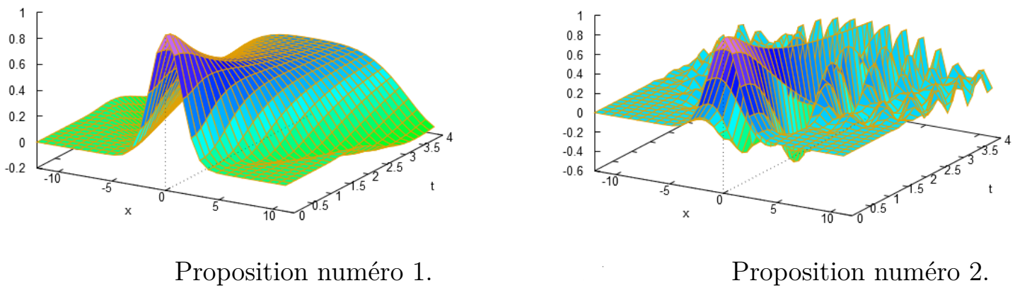
Voici deux graphiques qui représentent y(x ; t)y(x \,;\,t) avec x∈[−10 ; 10]x \in [-10 \,;\, 10] et t∈[0 ; 4]t \in [0 \,;\, 4] :

Laquelle de ces deux propositions graphiques correspond à la situation étudiée ? Justifier votre choix.

Correction
Parmi les deux graphiques qui ont proposés, celui qui correspond à notre situation c'est celui de la Proposition numéro 1 ; c'est le graphique de gauche.
En effet, il est le seul à mettre en évidence à l'instant initial t=0t = 0, une forme gaussienne centrée sur l'origine et strictement positive.
Cette gaussienne est lisse et à décroissance rapide ce qui lui assure d'appartenir à l'espace de Schwartz S(R)\mathcal{S}(\mathbb{R}).
Cela légitime, a priori, l'existence de la transformée de Fourier, ainsi que l'interversion des opérateurs de dérivation et d'intégration via le théorème de dérivation sous le signe intégral (somme de Lebesgue).

Signaler une erreur

Aide-nous à améliorer nos contenus en signalant les erreurs ou problèmes que tu penses avoir trouvés.

Connecte-toi ou crée un compte pour signaler une erreur.